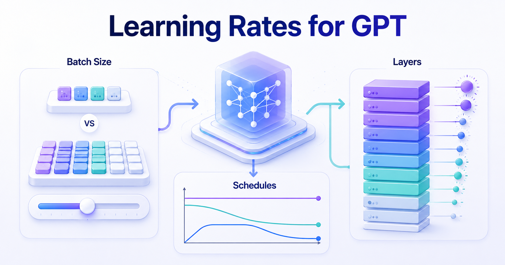
What batch size, decay schedules, and layer wise updates taught me about training a small GPT model
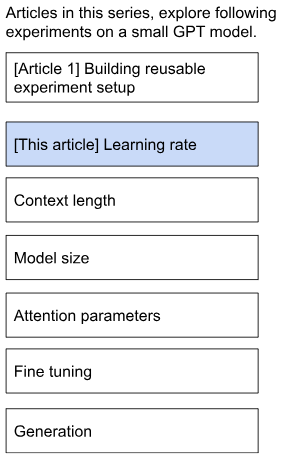
In the previous article, I tested a reusable experimentation framework with a small learning-rate sweep. Within the range I tried, higher learning rates produced lower validation loss—but the best result sat at the edge of the range.
That is usually the experiment’s polite way of saying, “Nice try, but you have not explored enough yet.”
Learning rate looks like a single configuration value: smaller values make cautious updates, while larger values make more aggressive ones. But recent research shows that its effect depends on much more—batch size, model size, training duration, decay strategy, optimizer choice, fine-tuning goals, and even the part of the model being updated.
I could not reproduce billion-parameter experiments on my local machine, so I used my smaller GPT model to explore three questions:
Does the useful learning-rate range change with batch size?
Should the learning rate remain constant or decay during training?
Should every part of the model use the same learning rate?
These experiments are not intended to validate the papers that inspired them. The goal is to use their questions to build a more practical intuition for what learning rate is actually doing.
Imagine a basketball coach helping a player correct a shot.
The learning rate is similar to the size of the correction after each attempt. A small correction might be, “Move your elbow slightly inward.” A large correction might be, “Change your entire shooting motion.”
Batch size determines how many shots the coach watches before providing feedback. With a batch size of two, the coach watches two shots and then suggests a change. With a batch size of eight, the coach watches eight shots before changing anything.
The larger batch provides a more stable view of the player’s shooting pattern, but the feedback arrives less frequently.
That creates an immediate question: should the size of each correction change when the model receives fewer updates?
I tested three batch sizes:
BATCH_SIZES = [2, 4, 8]
I kept the model architecture, dataset, random seed, optimizer, and evaluation approach constant.
I also gave every run approximately the same token budget. Each model processed roughly 100,000 training tokens, regardless of batch size.
This sounds fair, but it creates an important difference:
| Batch size | Approximate optimizer steps |
|---|---|
| 2 | 391 |
| 4 | 196 |
| 8 | 98 |
The batch-size-two model updated its parameters approximately four times as often as the batch-size-eight model. That difference became important when interpreting the results.
I explored the learning rate in three rounds.
The first round used relatively cautious values. The second moved higher, and the third deliberately entered the unstable region.
LEARNING_RATES = [
    1e-4, 3e-4, 1e-3,
    5e-3, 1e-2,
    5e-2, 1e-1, 5e-1,
]
The full experiment code creates one run for every batch-size and learning-rate combination:
experiment_grid = [
    (batch_size, learning_rate)
    for batch_size in BATCH_SIZES
    for learning_rate in LEARNING_RATES
]
Here are the final validation losses:
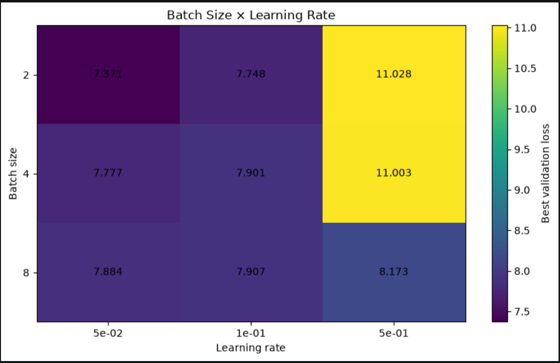
The overall pattern was surprisingly clean:
Too cautious → useful range → diminishing gains → instability
Increasing the learning rate helped at first. The improvement continued through 1e-3 and 5e-3, before beginning to flatten around 1e-2.
After that, the pattern reversed. At 5e-2, validation loss became worse. At 1e-1, training showed signs of instability. At 5e-1, the smaller-batch runs effectively broke down.
The best value I tested was 1e-2, but I would not describe it as a universally optimal learning rate. It was simply the strongest value for this model, dataset, optimizer, and training budget. Change those conditions, and the answer may also change.
Across the useful learning-rate range, batch size two frequently produced the lowest validation loss. Under the fixed token budget, the batch-size-two model received 391 opportunities to adjust its parameters, while the batch-size-eight model received only 98.
This does not prove that smaller batches are always better. It tells us that fixed tokens and fixed optimizer steps answer different questions.
A fixed-token experiment asks:
Which configuration learns more effectively from the same amount of data?
A fixed-step experiment asks:
Which configuration learns more effectively after the same number of parameter updates?
Under fixed steps, larger batches would process more total tokens. Under fixed tokens, smaller batches receive more updates.
Neither comparison is automatically more correct. The right comparison depends on which resource we are trying to hold constant.
The first experiment used a fixed learning rate, but training does not need equally large updates from beginning to end.
Early on, the model starts with mostly random parameters, so larger corrections can help. Later, smaller updates may help it settle instead of overshooting.
It is similar to coaching a basketball shot: first you fix the overall form, then you refine the wrist, release angle, and foot position.
That is the idea behind a learning-rate schedule. I compared three approaches:
Constant: After a short warmup, the learning rate stays at its peak value. It is simple, but updates may remain too aggressive near the end.
Cosine decay: The learning rate decreases smoothly after warmup, moving gradually from larger updates to smaller refinements.
Warmup–Stable–Decay: The rate warms up, stays stable through most of training, and decays only near the end.
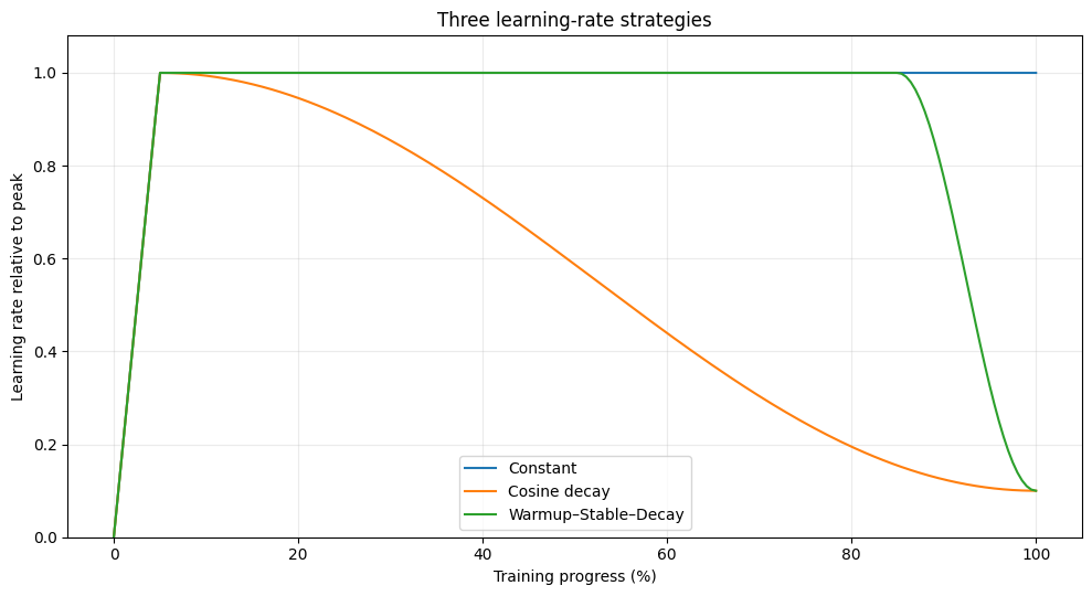
All three runs used the same model initialization, batch size, peak learning rate, and 200,000-token budget:
SCHEDULES = ["constant", "cosine", "wsd"]

BATCH_SIZE = 2
PEAK_LR = 5e-3
TOKEN_BUDGET = 200_000
The only variable was the schedule.'
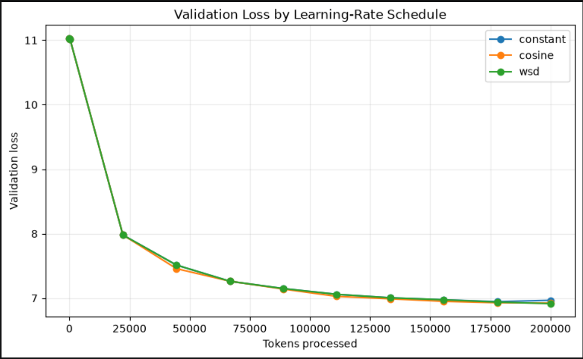
Both decay schedules achieved slightly lower validation loss than the constant schedule, supporting the idea that smaller late-stage updates can help the model settle.
But the differences were modest.
The bigger lesson was:
Choosing a good peak learning rate mattered more than choosing between the decay schedules.
There is also an important caveat. A schedule that produces the lowest pretraining loss may not produce the model that fine-tunes best later.
My experiment measured pretraining validation loss only, so it cannot answer that question. The “best” schedule therefore depends partly on what we plan to do with the model next.
So far, every part of the model used the same learning rate.
But a transformer contains embeddings, multiple transformer blocks, normalization layers, and an output projection. These components perform different jobs and may not respond equally to the same update size.
It is like giving the goalkeeper, striker, and defender exactly the same coaching instruction. Simple, but not always appropriate.
Supporting different learning rates across the model required changes to how the optimizer grouped and updated parameters. I will skip most of that implementation detail here, but the full code is available in the notebook:
View the full experiment notebook on GitHub
I tested three strategies.
Every parameter group used the same rate.
This is simple and common, but equal learning rates do not guarantee equal parameter movement.
Earlier layers received smaller rates, while deeper transformer blocks received progressively larger ones.
I treated this as a practical heuristic, not a rule that deeper layers should always learn faster.
Instead of assigning rates based on depth, I first ran a short 20-step calibration using a uniform learning rate.
Parameter groups that changed very little received a larger multiplier, while groups that changed aggressively received a smaller one. I capped the multipliers between 0.5 and 2.0 to avoid extreme adjustments.
Here is how the three strategies distributed the learning rate:
| Parameter group | Uniform | Depth-increasing | Update-balanced |
|---|---|---|---|
| Embeddings | 1.000 | 0.500 | 2.000 |
| Block 0 | 1.000 | 0.600 | 0.990 |
| Block 1 | 1.000 | 0.800 | 1.003 |
| Block 2 | 1.000 | 1.000 | 0.999 |
| Block 3 | 1.000 | 1.200 | 1.001 |
| Output | 1.000 | 1.000 | 0.500 |
Interestingly, the calibration did not recommend meaningfully different rates for the four transformer blocks.
The biggest corrections were elsewhere:
increase the embedding learning rate;
reduce the output learning rate.
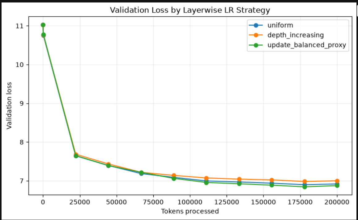
The update-balanced proxy performed best.
Unlike the depth heuristic, it focused its largest adjustments on the embeddings and output projection—the groups showing the biggest movement imbalance during calibration.
In this run, assigning learning rates based only on layer depth did not improve validation loss. The data-driven proxy performed better by responding to observed parameter movement instead of assuming that deeper layers always need larger updates.
That does not establish the proxy as a universally better strategy. It simply made the strongest recommendation for this particular run.
To compare the strategies, I measured each parameter group’s cumulative relative change:
||final parameters - initial parameters||
-----------------------------------------
       ||initial parameters||
A value of 1.0 means the group’s overall change norm was equal to its initial parameter norm. It does not mean that every individual parameter changed by 100%.
| Parameter group | Uniform | Depth-increasing | Update-balanced |
|---|---|---|---|
| Embeddings | 0.332 | 0.182 | 0.556 |
| Block 0 | 1.859 | 1.290 | 1.864 |
| Block 1 | 1.170 | 1.206 | 1.212 |
| Block 2 | 1.076 | 1.144 | 1.182 |
| Block 3 | 1.039 | 1.156 | 1.200 |
| Output | 5.255 | 5.309 | 3.763 |
The depth-increasing strategy made movement across the transformer blocks more balanced, but that did not translate into lower validation loss.
The update-balanced proxy did something different. It increased movement in the embeddings and reduced the unusually large movement in the output group.
This was a useful reminder that learning rate is only one factor affecting parameter movement. Gradient magnitude, parameter scale, AdamW’s adaptive updates, and weight decay also matter.
More balanced movement may help explain what is happening inside the model, but balance itself is not the objective. The optimizer is still trying to reduce loss—not make every layer change by a visually pleasing amount.
Although these were model-training experiments, five lessons felt familiar from product experimentation:
Start broad before optimizing narrowly. The difference between 1e-4 and 1e-2 was much larger than the difference between cosine and WSD. First find the region that works, then refine within it.
Define what a fair comparison means. Giving every batch size the same token budget also gave them different numbers of optimizer steps. A controlled experiment should match the question being asked, not simply make every number equal.
Inspect the mechanism, not only the headline metric. Validation loss showed which run performed better, while parameter movement explained how different parts of the model responded. Product metrics can similarly hide important differences in user behavior.
Do not overstate small differences. WSD performed best in this run, but its advantage over cosine was tiny. One experiment supports a local observation, not a universal rule.
Use part of the budget to reduce uncertainty. Short sweeps, proxy models, and even deliberately unstable runs can prevent expensive mistakes later. Sometimes the cheapest experiment is the one that tells us which costly experiment not to run.
Benchmarking Optimizers for Large Language Model Pretraining — Andrei Semenov, Matteo Pagliardini, and Martin Jaggi.
Scaling and Transferability of Annealing Strategies in Large Language Model Training — Siqi Wang et al.
Anytime Pretraining: Horizon-Free Learning-Rate Schedules with Weight Averaging — Alexandru Meterez et al.
Pre-training LLM without Learning Rate Decay Enhances Supervised Fine-Tuning — Kazuki Yano et al.
ScheduleFree+: Scaling Learning-Rate-Free & Schedule-Free Learning to Large Language Models — Aaron Defazio.
One LR Doesn’t Fit All: Heavy-Tail Guided Layerwise Learning Rates for LLMs — Di He et al.
On the Nonlinearity of Learning Rate Scaling for LLM Training — Zaiwen Yang et al.