保留正文与补采附件。源页面当前未重新核验;具体限制见交付清单。
 We value your privacy
We use cookies to enhance your browsing experience, serve personalised ads or content, and analyse our traffic. By clicking "Accept All", you consent to our use of cookies.
Customise Reject All Accept All
Customise Consent Preferences
 We use cookies to help you navigate efficiently and perform certain functions. You will find detailed information about all cookies under each consent category below.
The cookies that are categorised as "Necessary" are stored on your browser as they are essential for enabling the basic functionalities of the site. ... Show more
NecessaryAlways Active
Necessary cookies are required to enable the basic features of this site, such as providing secure log-in or adjusting your consent preferences. These cookies do not store any personally identifiable data.
-
Cookie
BCTempID
-
Duration
10 minutes
-
Description
No description available.
-
Cookie
__cf_bm
-
Duration
1 hour
-
Description
This cookie, set by Cloudflare, is used to support Cloudflare Bot Management.
-
Cookie
AWSALBCORS
-
Duration
7 days
-
Description
Amazon Web Services set this cookie for load balancing.
-
Cookie
_cfuvid
-
Duration
session
-
Description
Cloudflare sets this cookie to track users across sessions to optimize user experience by maintaining session consistency and providing personalized services
-
Cookie
li_gc
-
Duration
6 months
-
Description
Linkedin set this cookie for storing visitor's consent regarding using cookies for non-essential purposes.
-
Cookie
__hssrc
-
Duration
session
-
Description
This cookie is set by Hubspot whenever it changes the session cookie. The __hssrc cookie set to 1 indicates that the user has restarted the browser, and if the cookie does not exist, it is assumed to be a new session.
-
Cookie
__hssc
-
Duration
1 hour
-
Description
HubSpot sets this cookie to keep track of sessions and to determine if HubSpot should increment the session number and timestamps in the __hstc cookie.
-
Cookie
wpEmojiSettingsSupports
-
Duration
session
-
Description
WordPress sets this cookie when a user interacts with emojis on a WordPress site. It helps determine if the user's browser can display emojis properly.
-
Cookie
BCSessionID
-
Duration
1 year 1 month 4 days
-
Description
Blueconic sets this cookie as a unique identifier for the BlueConic profile.
-
Cookie
_octo
-
Duration
1 year
-
Description
No description available.
-
Cookie
logged_in
-
Duration
1 year
-
Description
No description available.
-
Cookie
__Secure-YEC
-
Duration
past
-
Description
YouTube sets this cookie to stores the user's video player preferences using embedded YouTube video
-
Cookie
__eoi
-
Duration
6 months
-
Description
Description is currently not available.
-
Cookie
AWSALBTGCORS
-
Duration
7 days
-
Description
No description available.
-
Cookie
login-status-p
-
Duration
past
-
Description
Description is currently not available.
-
Cookie
AWSALBTG
-
Duration
7 days
-
Description
No description available.
-
Cookie
csrf_token
-
Duration
session
-
Description
No description available.
-
Cookie
token_v2
-
Duration
1 day
-
Description
Description is currently not available.
-
Cookie
D
-
Duration
1 year
-
Description
Description is currently not available.
-
Cookie
PHPSESSID
-
Duration
session
-
Description
This cookie is native to PHP applications. The cookie stores and identifies a user's unique session ID to manage user sessions on the website. The cookie is a session cookie and will be deleted when all the browser windows are closed.
-
Cookie
VISITOR_PRIVACY_METADATA
-
Duration
6 months
-
Description
YouTube sets this cookie to store the user's cookie consent state for the current domain.
-
Cookie
cookietest
-
Duration
session
-
Description
The cookietest cookie is typically used to determine whether the user's browser accepts cookies, essential for website functionality and user experience.
-
Cookie
__Host-airtable-session
-
Duration
1 year
-
Description
This cookie is used to enable us to integrate the services of Airtable.
-
Cookie
__Host-airtable-session.sig
-
Duration
1 year
-
Description
This cookie is used to enable us to integrate the services of Airtable.
-
Cookie
m
-
Duration
1 year 1 month 4 days
-
Description
Stripe sets this cookie for fraud prevention purposes. It identifies the device used to access the website, allowing the website to be formatted accordingly.
-
Cookie
BIGipServer*
-
Duration
session
-
Description
Marketo sets this cookie to collect information about the user's online activity and build a profile about their interests to provide advertisements relevant to the user.
-
Cookie
__cfruid
-
Duration
session
-
Description
Cloudflare sets this cookie to identify trusted web traffic.
-
Cookie
_GRECAPTCHA
-
Duration
6 months
-
Description
Google Recaptcha service sets this cookie to identify bots to protect the website against malicious spam attacks.
-
Cookie
__Secure-YNID
-
Duration
6 months
-
Description
Google cookie used to protect user security and prevent fraud, especially during the login process.
-
Cookie
cookieyes-consent
-
Duration
1 year
-
Description
CookieYes sets this cookie to remember users' consent preferences so that their preferences are respected on subsequent visits to this site. It does not collect or store any personal information about the site visitors.
Functional
Functional cookies help perform certain functionalities like sharing the content of the website on social media platforms, collecting feedback, and other third-party features.
-
Cookie
lidc
-
Duration
1 day
-
Description
LinkedIn sets the lidc cookie to facilitate data center selection.
-
Cookie
brw
-
Duration
1 year
-
Description
No description available.
-
Cookie
brwConsent
-
Duration
5 minutes
-
Description
Description is currently not available.
-
Cookie
WMF-Uniq
-
Duration
1 year
-
Description
Description is currently not available.
-
Cookie
loom_anon_comment
-
Duration
1 year
-
Description
No description available.
-
Cookie
loom_referral_video
-
Duration
session
-
Description
Description is currently not available.
-
Cookie
VISITOR_INFO1_LIVE
-
Duration
6 months
-
Description
A cookie set by YouTube to measure bandwidth that determines whether the user gets the new or old player interface.
-
Cookie
yt-remote-connected-devices
-
Duration
Never Expires
-
Description
YouTube sets this cookie to store the user's video preferences using embedded YouTube videos.
-
Cookie
ytidb::LAST_RESULT_ENTRY_KEY
-
Duration
Never Expires
-
Description
The cookie ytidb::LAST_RESULT_ENTRY_KEY is used by YouTube to store the last search result entry that was clicked by the user. This information is used to improve the user experience by providing more relevant search results in the future.
-
Cookie
yt-remote-device-id
-
Duration
Never Expires
-
Description
YouTube sets this cookie to store the user's video preferences using embedded YouTube videos.
-
Cookie
yt-remote-session-name
-
Duration
session
-
Description
The yt-remote-session-name cookie is used by YouTube to store the user's video player preferences using embedded YouTube video.
-
Cookie
yt-remote-fast-check-period
-
Duration
session
-
Description
The yt-remote-fast-check-period cookie is used by YouTube to store the user's video player preferences for embedded YouTube videos.
-
Cookie
yt-remote-session-app
-
Duration
session
-
Description
The yt-remote-session-app cookie is used by YouTube to store user preferences and information about the interface of the embedded YouTube video player.
-
Cookie
yt-remote-cast-available
-
Duration
session
-
Description
The yt-remote-cast-available cookie is used to store the user's preferences regarding whether casting is available on their YouTube video player.
-
Cookie
yt-remote-cast-installed
-
Duration
session
-
Description
The yt-remote-cast-installed cookie is used to store the user's video player preferences using embedded YouTube video.
-
Cookie
cp_session
-
Duration
3 months
-
Description
Codepen sets this cookie for Help systems found in the website.
-
Cookie
loid
-
Duration
1 year 1 month 4 days
-
Description
This cookie is set by the Reddit. The cookie enables the sharing of content from the website onto the social media platform.
Analytics
Analytical cookies are used to understand how visitors interact with the website. These cookies help provide information on metrics such as the number of visitors, bounce rate, traffic source, etc.
-
Cookie
__hstc
-
Duration
6 months
-
Description
Hubspot set this main cookie for tracking visitors. It contains the domain, initial timestamp (first visit), last timestamp (last visit), current timestamp (this visit), and session number (increments for each subsequent session).
-
Cookie
hubspotutk
-
Duration
6 months
-
Description
HubSpot sets this cookie to keep track of the visitors to the website. This cookie is passed to HubSpot on form submission and used when deduplicating contacts.
-
Cookie
_ga
-
Duration
1 year 1 month 4 days
-
Description
Google Analytics sets this cookie to calculate visitor, session and campaign data and track site usage for the site's analytics report. The cookie stores information anonymously and assigns a randomly generated number to recognise unique visitors.
-
Cookie
ga*
-
Duration
1 year 1 month 4 days
-
Description
Google Analytics sets this cookie to store and count page views.
-
Cookie
__Host-psifi.analyticsTrace
-
Duration
6 hours
-
Description
Description is currently not available.
-
Cookie
__Host-psifi.analyticsTraceV2
-
Duration
6 hours
-
Description
Description is currently not available.
-
Cookie
_gh_sess
-
Duration
session
-
Description
GitHub sets this cookie for temporary application and framework state between pages like what step the user is on in a multiple step form.
-
Cookie
YSC
-
Duration
session
-
Description
YSC cookie is set by Youtube and is used to track the views of embedded videos on Youtube pages.
-
Cookie
ajs_anonymous_id
-
Duration
1 year
-
Description
This cookie is set by Segment to count the number of people who visit a certain site by tracking if they have visited before.
-
Cookie
vuid
-
Duration
1 year 1 month 4 days
-
Description
Vimeo installs this cookie to collect tracking information by setting a unique ID to embed videos on the website.
Performance
Performance cookies are used to understand and analyse the key performance indexes of the website which helps in delivering a better user experience for the visitors.
-
Cookie
AWSALB
-
Duration
7 days
-
Description
AWSALB is an application load balancer cookie set by Amazon Web Services to map the session to the target.
-
Cookie
acq
-
Duration
past
-
Description
Description is currently not available.
-
Cookie
acq.sig
-
Duration
past
-
Description
Description is currently not available.
-
Cookie
ptc
-
Duration
2 years
-
Description
No description available.
Advertisement
Advertisement cookies are used to provide visitors with customised advertisements based on the pages you visited previously and to analyse the effectiveness of the ad campaigns.
-
Cookie
muc_ads
-
Duration
1 year 1 month 4 days
-
Description
Twitter sets this cookie to collect user behaviour and interaction data to optimize the website.
-
Cookie
guest_id_marketing
-
Duration
1 year 1 month 4 days
-
Description
Twitter sets this cookie to identify and track the website visitor.
-
Cookie
guest_id_ads
-
Duration
1 year 1 month 4 days
-
Description
Twitter sets this cookie to identify and track the website visitor.
-
Cookie
personalization_id
-
Duration
1 year 1 month 4 days
-
Description
Twitter sets this cookie to integrate and share features for social media and also store information about how the user uses the website, for tracking and targeting.
-
Cookie
guest_id
-
Duration
1 year 1 month 4 days
-
Description
Twitter sets this cookie to identify and track the website visitor. It registers if a user is signed in to the Twitter platform and collects information about ad preferences.
-
Cookie
bcookie
-
Duration
1 year
-
Description
LinkedIn sets this cookie from LinkedIn share buttons and ad tags to recognize browser IDs.
-
Cookie
__Secure-ROLLOUT_TOKEN
-
Duration
6 months
-
Description
YouTube sets this cookie to manage feature rollout and experimentation. It helps Google control which new features or interface changes are shown to users as part of testing and staged rollouts, ensuring consistent experience for a given user during an experiment.
-
Cookie
yt.innertube::nextId
-
Duration
Never Expires
-
Description
YouTube sets this cookie to register a unique ID to store data on what videos from YouTube the user has seen.
-
Cookie
yt.innertube::requests
-
Duration
Never Expires
-
Description
YouTube sets this cookie to register a unique ID to store data on what videos from YouTube the user has seen.
-
Cookie
session_tracker
-
Duration
session
-
Description
This cookie is set by the Reddit. This cookie is used to identify trusted web traffic. It also helps in adverstising on the website.
-
Cookie
edgebucket
-
Duration
session
-
Description
Reddit sets this cookie to save the information about a log-on Reddit user, for the purpose of advertisement recommendations and updating the content.
-
Cookie
did
-
Duration
1 year
-
Description
Arbor sets this cookie to show targeted ads to site visitors.This cookie expires after 2 months or 1 year.
Uncategorised
Other uncategorised cookies are those that are being analysed and have not been classified into a category as yet.
No cookies to display.
Reject All Save My Preferences Accept All
Toggle SearchToggle Mobile Navigation
Publish AI, ML & data-science insights to a global community of data professionals.
Sign inSubmit an Article
LatestEditor's PicksNewsletterShipAI
Write For TDS
LinkedInXToggle Search
Data Science
Ridge, LASSO, and ElasticNet Regression
The continuing adventures of regularization and the eternal quest to prevent model overfitting!
James Andrew Godwin
April 2, 202119 min read
 LASSO, Ridge, and Elasticnet regression | Photo by Daniele Levis Pulusi
This article is a continuation of last week's intro to regularization with linear regression. Lettuce yonder back into the nitty-gritty of making the best data science/ machine learning models possible with more advanced techniques on simplifying our models. How do we simplify our models? By removing as many features as possible. Why do I want to do this? I want to have a simpler model. Why do I want a simpler model? Well, because a simpler model generalizes better. What does generalization mean? It means that you can actually use it in the real world. The model does not just explain the training data but it also has a better chance of explaining data that we have not seen before.
Learn this step by step with the interactive AI and Data Scientist and Machine Learning roadmaps.
Regularization
Regularization seeks to control variance by adding a tuning parameter, lambda, or alpha:
LASSO (L1 regularization)
- regularization term penalizes absolute value of the coefficients
- sets irrelevant values to 0
- might remove too many features in your model
Ridge regression (L2 regularization)
- penalizes the size (square of the magnitude) of the regression coefficients
- enforces the B (slope/partial slope) coefficients to be lower, but not 0
- does not remove irrelevant features, but minimizes their impact
Now do not worry about that lambda. For right now assume lambda is one. For ridge regression, we penalize the size of the regression coefficient. So a larger regression coefficient is a larger penalty.
 b and c are the regression coefficients
So in this ridge regression, I would take the square of b and add it to the square of c. And that would be my penalty. Now it is slightly more complex than that because sometimes I want to do make the penalty stronger or less strong, I now introduce this lambda, this tuning parameter. So my penalty now becomes:
 Otherwise known as the L2 or Euclidian norm
So this is what the Ridge regression does. By adding this penalty to my cost function, during training, it's going to keep these b's and these c's small. And by doing so this is going to simplify the model; that means any given column is not going to have that much power.
LASSO does pretty much the same thing. Except for the regularization penalty is without the square:
 Otherwise known as the L1 or Manhattan/taxicab norm
Please take note that because you could have negative values here, so you need to add an absolute value on the coefficients, on the partial slopes.
The coefficients b, and c, in the above example, are adjusted by the algorithm you are using. We add another quirk to it by introducing a lambda penalty that is not 1 - it has always been there behind the scenes but we kept it at 1 for simplicity. When it comes time to evaluate the goodness of your model, through the cost function, we are going to multiply a penalty we called lambda to your coefficients (or to the square of your coefficients), and that will be an additional penalty.
We still have our general cost function. This is just an addition to that cost function. Our general cost function is always the same and it is the one where we have y - predicted y and take the square of that and sum all those up. So that is our cost function, the baseline. Now, the additional penalty in order to regularize is either this Ridge regression, which uses the so-called L2 norm, or the LASSO (least absolute shrinkage and selection operator) regression, which uses the so-called L1 norm.
For both types of regression, a larger coefficient penalizes the model. With Ridge, the penalty is disproportionately larger because of the square, but in general, a larger coefficient reduces model performance, a larger coefficient reduces the goodness of fit.
N.B: The L notation is a reference to Minkowski norms and Lp spaces. These just generalize the notion of taxicab and Euclidean distances to p >0p>0 in the following expression:
 For those of you who remember back to Linear Algebra
Ridge regression
Reiterating again, Ridge regression is a way to limit the number of independent variables (columns/features/attributes) in the regression. The regular least-squares criterion minimizes the least-squares of the error plus a regularization term that is a product of a constant and the sum of squared coefficients:
 Ridge regression cost function, expressed another way | alpha is sometimes used instead of lambda in certain literature
Essentially this is preventing the partial slope terms from getting too large.
Here I am calling this penalty coefficient alpha as opposed to lambda. And this is a little bit confusing since alpha has a few meanings that are very closely related in this jargon. So just want to warn you, in general, you might have some problems, lambda is a safe bet. Alpha has at least two very closely, but still different meanings.
Here, we have this beta squared. What is beta? Beta is a vector of your coefficients. So beta is a vector that is basically in my would have been b and c in my previous example. Remember, I had y = a +b X1 + c X2, b and c were two coefficients. Beta is a vector, and here composed of two numbers. In my example, those two numbers are b and c; a is the intercept, sometimes confusingly referred to as b.
So beta squared is exactly the same thing as the equation above. What is a partial slope? Another word for partial slope is a coefficient. Why do we call it a partial slope? Well, if you remember, we have a slope when we have a linear regression, y = a + b X, b is the slope. Well, if you have multiple x's, so y = a + b X1 + c X2 + d X3 and so on and so on. Then, in my example, that I just mentioned b, c, and d are all partial slopes, that is because they are multiplied by the columns. And the way the input value from the column changes from those variables change will affect the output. And it will affect it more if that coefficient or that partial slope is greater. When I say greater, I mean in magnitude.
So the Ridge objective *is the residual sum of squares (RSS) +lambda (sum of squares of the coefficients)**.
- use lambda to balance minimizing RSS vs. minimizing the coefficients
- when lambda = 0, results are the same as regular linear regression: you have removed the Ridge regression penalty
- as lambda increases to infinity, coefficients become closer to 0
- any non-zero lambda value will shrink the coefficients to be smaller than with non-regularized regression
- as lambda (alpha) increases, model complexity decreases
Lambda is just a scalar that should be learned from your data using cross-validation (tuning). So lambda is always positive and is between zero and infinity. And just to give you a basic idea of its range, it is rarely much larger than one, maybe going to two or three, and often is a small fraction of one. Why is that? Well, that is just the way things work out. There exist counterexamples to what I just said, but as a general heuristic, what you generally find is that the lambda is between zero and, and a small value, let us say roughly two.
If the model complexity decreases as lambda increases, how can you see this?
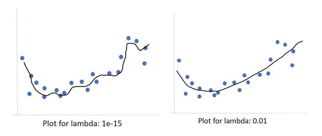 Our regression lines fit the blue dots well
In the example fits above I approximate some form of regression, in this case, probably not a linear regression. And that regression worked pretty well. And then we added the lambda parameter. And hopefully, things got better. If I were to eyeball this here, I would probably want the one on the right. My rationale is, I see these blue dots, they are flying all over the place, they are up and down above and beneath that black line. I expect there to be overall, more variation in where those blue dots can land, a lot of variation. And so I think that trying to find the model that tries to minimize the residuals of these blue dots will try to minimize it too much, what will happen is it will become too complex of a model, it will overfit. And then when new data comes by, data that the model has never seen, that new data is not going to be there where this model is fitting.
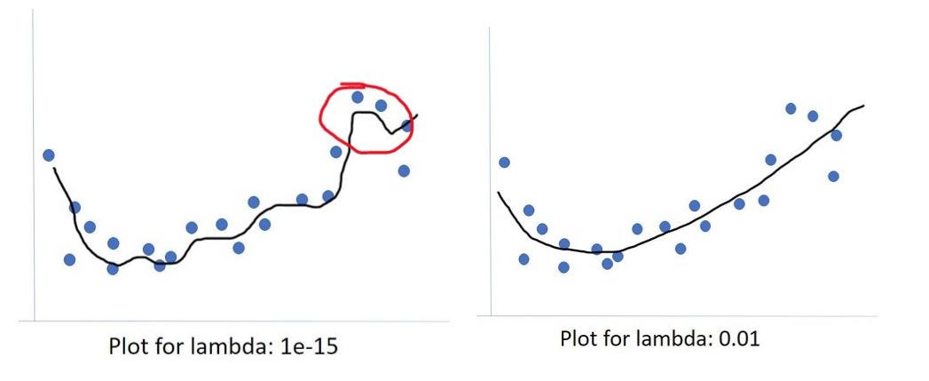 The red circle is likely overfitting the residuals
So for instance, this little quirk circled in red, looks pretty good. But my guess is that is just because one or two data points had these high y values relatively - high y values. Methinks that was just a quirk. Probably this should just go straight over, as it does on the right-most image. Because if I look at how much overall these blue points are going up and down, I cannot really justify creating a model that is trying to go down to catch to minimize the residual of this one bluepoint and then going right back up. As such, the small lambda value is likely overfitting and I believe that the 1/100 lambda value on the right actually fits the data much better and will generalize better.
LASSO
LASSO regression does pretty much the same thing; it is another way to limit the number of independent variables in the regression. The only difference is, it uses the absolute value. Now the thing is that because of the math, what it does is not just reduce the coefficients, LASSO actually removes the coefficients. Many people like LASSO for this reason: the coefficients can actually go to zero, whereas in the Ridge regression, they do not go to zero, they become small, but they never vanish.
Now, you can always help the last way, if you see that coefficient has gotten really small, you can just say, "Okay, I'm going to just toss this column, because it has such a small coefficient." What is nice about LASSO is that it will actually do that for you in an intelligent way.
 y is the predicted for j points, there are i terms with beta coefficients - lambda limits the betas
Beta a vector of your coefficients. Instead of squaring them, you just take the absolute value.
Linear algebra
Next is a quick review of linear algebra. Why do we have a quick review of linear algebra? Well, because machine learning is a lot of linear algebra and the more you understand about the machine learning algorithms, the often the better you can apply them. When studying data science, you are not studying machine learning, you are studying how to use the machine learning algorithms.
Algebraic properties of matrices:
- add/subtract matrices: must be of the same dimensions (m * n)
- for multiplication of matrices: inner dimensions must match
- remember that matrix multiplication is not commutative: A x B != B x A
- a matrix multiplied by its inverse yields the identity matrix
- matrix division is not defined
Linear regression with matrices
Consider the linear regression formula:
 written as a matrix:
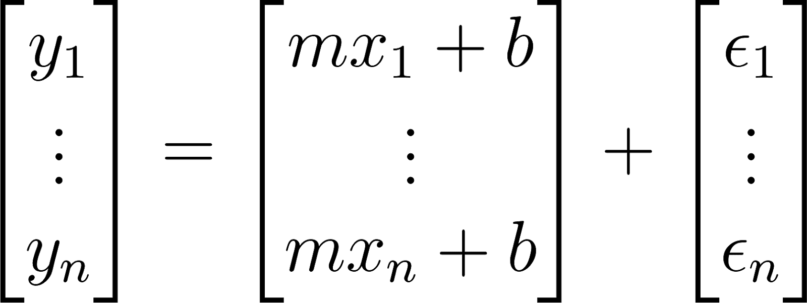 which can be rewritten as:
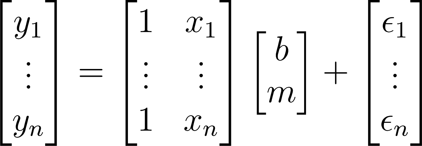 For linear regression with matrices, if you have, say 10 cases, that means 10 points and you will have 10 columns, then there will be an exact, best solution. There will be a simple solution to that. However, not in every case, there are cases where you have colinearity, which means when one column is basically the same as another column or the same as a combination of some other columns. When this occurs you generally have infinitely many solutions. And we do not like this because having infinitely many solutions, means you do not have any useful solutions. If then there are situations where there is simply no solution can occur. But the general case or the case that you hope for is that you have exactly one good solution.
Most of the time, when we do machine learning, or data science is we have many more cases than we have variables; we have many more data points than we have columns; we have many more rows than we have columns - I am just repeating the same thing over and over with slightly different words. This is going to cause us an issue, for one thing, that means our matrix of x is not a square matrix.
So when we want to invert it, and I will show you that we will want to do that, it is going to cause us some problems, along with colinearity and stuff like that.
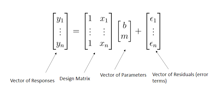 Succinctly: y = X * Beta + Epsion
These concepts are best demonstrated in code.
Python example: Singular value decomposition
Previously, I mentioned stepwise regression as a way to regularize, by finding meaningful features one at a time, either by the forward or backward methodology. I now introduce singular value decomposition (SVD) as another meaningful way to find features.
Regularization methods stabilize the inverse of the model matrix. We will use the SVD method to stabilize a model matrix.
N.B: Stepwise regression is a computationally-intensive process since we must recompute the model many times. There are methods that allow computation of the updated model, but with a large number of features, there are numerous permutations. We need methods that can handle hundreds, thousands, or even millions of features. Consider a small data set with only 20 features. The amount of possible linear models with NO interaction terms is given by:
 Which is the sum of the 21st row of Pascal's triangle. This comes out to be:
 Although according to our algorithm, this would be the maximum number of models to compute, you can see how computationally hard this becomes when naively considering stepwise regression.
In order to understand the motivation and methods of feature selection/transformation, I will review some linear algebra.
Linear algebra review
text
import numpy as np
text
a_list = [2]*3
print(a_list)
print(type(a_list))
a = np.array([2]*3)
print(a)
print(type(a))
b = np.arange(1, 4)
print(b)
print(type(b))
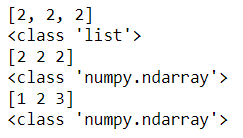 Jupyter displays lists and arrays similarly
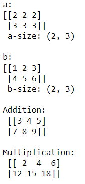
Matrix multiplication and addition
text
a2d = np.array([[2]*3, [3]*3])
print('a: n{} n a-size: {}'.format(a2d, a2d.shape))
b2d = np.reshape(np.arange(1,7), newshape=(2, 3))
print('nb: n{} n b-size: {}'.format(b2d, b2d.shape))
text
# Addition
print('nAddition: n {}'.format(a2d + b2d))
# Multiplication
print('nMultiplication: n {}'.format(a2d * b2d))
Matrix transposition
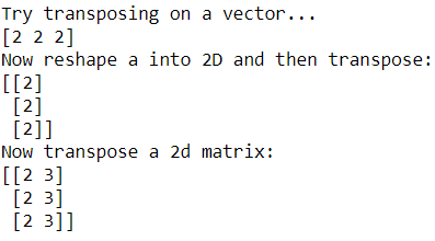
We can also transpose a two-dimensional matrix by flipping the rows and columns. We use the numpy method np.transpose.
text
print('Try transposing on a vector...')
print(np.transpose(a))
# Transposition on a vector does not work
text
print('Now reshape a into 2D and then transpose:')
print(np.transpose(np.reshape(a, newshape=(1,3))))
print('Now transpose a 2d matrix:')
print(np.transpose(a2d))
Matrix dot product
We need to know how to compute the dot product , which is also known as the scalar product or inner product of two vectors of equal length, via element-wise multiplication then summing them all up:
 text
print('np.dot(a, b) = np.dot({}, {})'.format(a, b))
np.dot(a, b)
 The square root of the inner product of a vector with itself is the length or L2 norm of the vector:
 We can also write the inner product as:


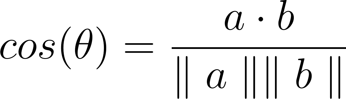 Notice that the inner product of orthogonal vectors is 0
text
aa = np.array([1, 0, 0])
bb = np.array([0, 1, 1])
print(inner_prod(aa, bb))
 Linearly independent vectors are completely orthogonal
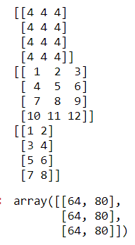
Here are some operations on matrices. Let A and B be m=4 rows by n=3 columns matrices:
text
A = np.array([[4]*3]*4)
print(A)
B = np.array(np.reshape(np.arange(1, 13), newshape = (4, 3)))
print(B)
C = np.array(np.reshape(np.arange(1, 9), newshape = (4, 2)))
print(C)
np.dot(np.transpose(A), C)
Identity matrix
This special, square matrix has ones on the diagonal and zeros elsewhere:
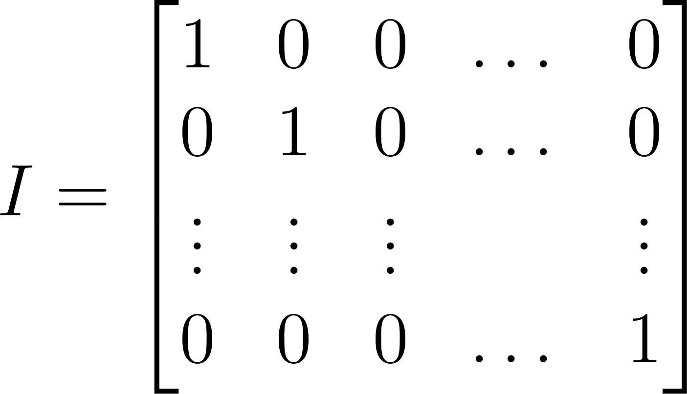 The matrix equivalent of 1
The identity multiplied by any matrix gives that matrix. If AB is a rectangular matrix then:
 In
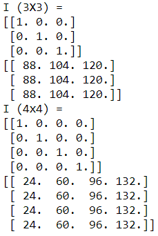
numpy the Identity matrix is called np.eye and takes as an argument the number of rows/columns:
text
I3 = np.eye(3)
I4 = np.eye(4)
text
print('I (3X3) = n{}'.format(I3))
print(np.dot(I3, AtB))
text
print('I (4x4) = n{}'.format(I4))
print(np.dot(I4, ABt))
Inverse of a matrix
Define and compute an inverse of a matrix such that:


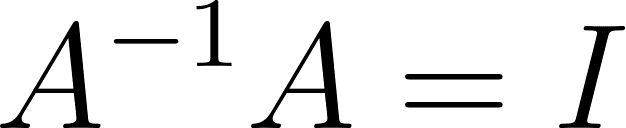 Use the Linear Algebra methods in
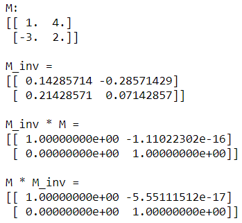
numpy to get the inverse of matrix M with np.linalg.inv
text
M = np.array([[1., 4.], [-3., 2.]])
M_inverse = np.linalg.inv(M)
text
print('M: n{}'.format(M))
print('nM_inv = n{}'.format(M_inverse))
print('nM_inv * M = n{}'.format(np.dot(M_inverse, M)))
print('nM * M_inv = n{}'.format(np.dot(M, M_inverse)))
 With this brief refresher aside, we can now jump into regularizing models with SVD.
Singular Value Decomposition
In machine learning, we often encounter matrices that cannot be inverted directly. Instead, we need a decomposition of A that allows us to compute A^−1, which we can do with SVD:

- U is the orthogonal unit norm left singular vectors
- V is the orthogonal unit norm right singular vectors, and V∗ is the conjugate transpose; for real-valued A this is just VT
- D is a diagonal matrix of singular values, which are said to define a spectrum
- A is comprised of the linear combination of singular vectors scaled by singular values
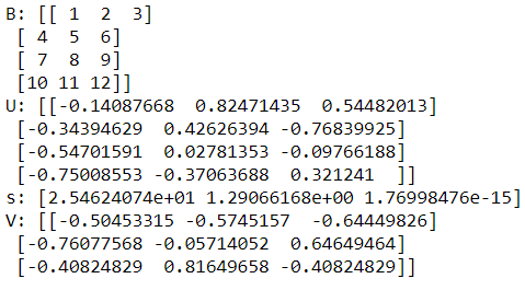
To compute the SVD of a matrix and view the results execute the code in the cell below. We use the numpy method called np.linalg.svd using s for the singular values:
text
U, s, V = np.linalg.svd(B, full_matrices=False)
print('B: {}'.format(B)) # ESHx
print('U: {}'.format(U))
print('s: {}'.format(s))
print('V: {}'.format(V))
Regularization with Ridge and Lasso Regression
So far, we have looked at two approaches for dealing with over-parameterized models; feature selection by stepwise regression and singular value decomposition. In this section, we will explore the most widely used regularization method for optimization-based machine learning models, Ridge regression.
Let's start by examining the matrix-equation formulation of the linear regression problem. The goal is to compute a vector of model coefficients or weights which minimize the mean squared residuals, given a vector of data 𝑥x and a model matrix A. We can express our model as:
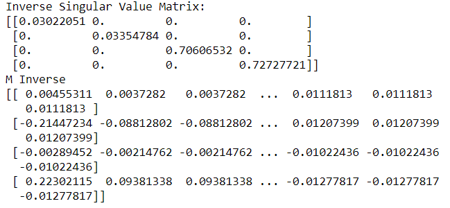
 Execute the code in the cell below which computes the (𝐴^𝑇 𝐴+𝜆²)^-1 A^T matrix with a lambda value of 0.1``
text
U, s, V = np.linalg.svd(M, full_matrices=False)
text
# Calculate the inverse singular value matrix from SVD
lambda_val = 1.0
d = np.diag(1. / (s + lambda_val))
text
print('Inverse Singular Value Matrix:')
print(d)
text
# Compute pseudo-inverse
mInv = np.dot(np.transpose(V), np.dot(d, np.transpose(U)))
text
print('M Inverse')
print(mInv)
Bias-variance trade-off
The bias-variance trade-off is a fundamental property of machine learning models. To understand this trade-off let's decompose the mean square error for a model as follows:
 Regularization will reduce variance, but increases bias. Regularization parameters are chosen to minimize delta_X. In many cases, this process proves challenging, involving significant time-consuming trial and error.
The irreducible error is the limit of model accuracy. Even if you had a perfect model with no bias or variance, the irreducible error is inherent in the data and model. You cannot do better.
The
statsmodels package allows us to compute a sequence of Ridge regression solutions. The function that does this uses a method called 'Elasticnet', know that ridge regression is a specific case of elastic-net, and I will talk more about this later.
N.B: This is a continuation of my previous work on the Galton family dataset.
The code in the cell below computes solutions for 20 values of lambda:
text
# Ridge regression with various penalties in Statsmodels
# sequence of lambdas
log_lambda_seq = np.linspace(-6, 2, 50)
lambda_seq = np.exp(log_lambda_seq)
text
coeffs_array = []
rsq_array = []
formula = 'childHeight ~ mother + father + mother_sqr + father_sqr + 1'
text
for lamb in lambda_seq:
 ridge_model = sm.ols(formula, data=male_df).fit_regularized(method='elastic_net', alpha=lamb, L1_wt=0)
 coeffs_array.append(list(ridge_model.params))
 predictions = ridge_model.fittedvalues
 residuals = [x - y for x, y in zip(np.squeeze(predictions), childHeight)]
text
SSR = np.sum(np.square(residuals))
 SST = np.sum(np.square(childHeight - np.mean(childHeight)))
text
rsq = 1 - (SSR / SST)
 rsq_array.append(rsq)
text
# pull out partial slopes (drop intercept version)
beta_coeffs = [x[1:] for x in coeffs_array]
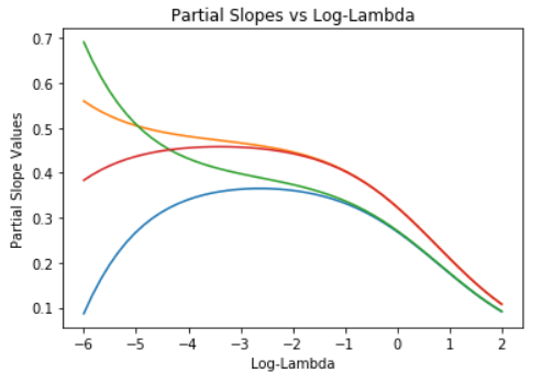
plt.plot(log_lambda_seq, beta_coeffs)
plt.title('Partial Slopes vs Log-Lambda')
plt.ylabel('Partial Slope Values')
plt.xlabel('Log-Lambda')
plt.show()
 Plot partial slopes vs R²:
text
# % deviance explained
plt.plot(rsq_array, beta_coeffs)
plt.xlim([0.0, 0.25])
plt.title('Partial Slopes vs Log-Lambda')
plt.xlabel('R-squared')
plt.ylabel('Partial Slopes')
plt.show()
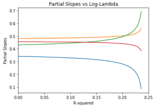 Notice that as lambda increases, the values of the 4 model coefficients decrease toward zero. When all coefficients are zero, the model predicts all values of the label as zero! In other words, high values of lambda give highly biased solutions, but with very low variance.
For small values of lambda, the situation is just the opposite. The solution has a low bias, but is quite unstable, having maximum variance. This bias-variance trade-off is a key concept in machine learning.
LASSO regression
We can also do regularization using other norms. LASSO or L1 regularization limits the sum of the absolute values of the model coefficients. The L1 norm is sometimes known as the Manhattan norm since distances are measured as if you were traveling on a rectangular grid of streets.
You can also think of LASSO regression as limiting the L1 norm of the values of the model coefficient vector. The value of lambda determines how much the norm of the coefficient vector constrains the solution.
Performing the same calculations as before, but with a different regularization norm and associated penalty:
text
# LASSO regression with a sequence of lambdas
# sequence of lambdas
log_lambda_seq = np.linspace(-6, 2, 50)
lambda_seq = np.exp(log_lambda_seq)
text
coeffs_array = []
rsq_array = []
formula = 'childHeight ~ mother + father + mother_sqr + father_sqr + 1'
text
for lamb in lambda_seq:
 ridge_model = sm.ols(formula, data=male_df).fit_regularized(method='elastic_net', alpha=lamb, L1_wt=1)
 coeffs_array.append(list(ridge_model.params))
 predictions = ridge_model.fittedvalues
 residuals = [x - y for x, y in zip(np.squeeze(predictions), childHeight)]
text
SSR = np.sum(np.square(residuals))
 SST = np.sum(np.square(childHeight - np.mean(childHeight)))
text
rsq = 1 - (SSR / SST)
 rsq_array.append(rsq)
text
# drop intercept version
beta_coeffs = [x[1:] for x in coeffs_array]
plt.plot(log_lambda_seq, beta_coeffs)
plt.title('Partial Slopes vs Log-Lambda')
plt.ylabel('Partial Slope Values')
plt.xlabel('Log-Lambda')
plt.show()
 text
# plot partial slopes vs R squared (% deviance explained)
plt.plot(rsq_array, beta_coeffs)
plt.xlim([0.0, 0.25])
plt.title('Partial Slopes vs Log-Lambda')
plt.xlabel('R-squared')
plt.ylabel('Partial Slopes')
plt.show()
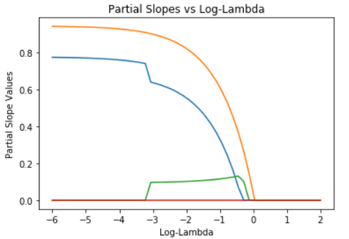
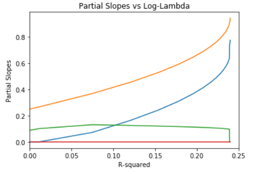 Notice that model coefficients are much more tightly constrained than for L2 regularization. In fact, only two of the possible model coefficients have non-zero values at all! This is typical of L1 or LASSO regression.
Elastic Net regression
The elastic net algorithm uses a weighted combination of L1 and L2 regularization. As you can probably see, the same function is used for LASSO and Ridge regression with only the L1_wt argument changing. This argument determines how much weight goes to the L1-norm of the partial slopes. If the regularization is pure L2 (Ridge) and if L1_wt = 1.0 the regularization is pure L1 (LASSO).
The code in the cell below gives equal weight to each regression method. Execute this code and examine the results:
text
# ElasticNet Regression with a sequence of lambdas
# sequence of lambdas
log_lambda_seq = np.linspace(-6, 0, 50)
lambda_seq = np.exp(log_lambda_seq)
text
coeffs_array = []
rsq_array = []
formula = 'childHeight ~ mother + father + mother_sqr + father_sqr + 1'
text
for lamb in lambda_seq:
 ridge_model = sm.ols(formula, data=male_df).fit_regularized(method='elastic_net', alpha=lamb, L1_wt=0.75)
 coeffs_array.append(list(ridge_model.params))
 predictions = ridge_model.fittedvalues
 residuals = [x - y for x, y in zip(np.squeeze(predictions), childHeight)]
text
SSR = np.sum(np.square(residuals))
 SST = np.sum(np.square(childHeight - np.mean(childHeight)))
text
rsq = 1 - (SSR / SST)
 rsq_array.append(rsq)
text
# pull out partial slopes (drop intercept version)
beta_coeffs = [x[1:] for x in coeffs_array]
plt.plot(log_lambda_seq, beta_coeffs)
plt.title('Partial Slopes vs Log-Lambda')
plt.ylabel('Partial Slope Values')
plt.xlabel('Log-Lambda')
plt.show()
 text
# plot partial slopes vs R squared (% deviance explained)
plt.plot(rsq_array, beta_coeffs)
plt.xlim([0.0, 0.25])
plt.title('Partial Slopes vs Log-Lambda')
plt.xlabel('R-squared')
plt.ylabel('Partial Slopes')
plt.show()
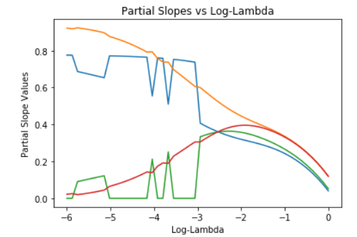
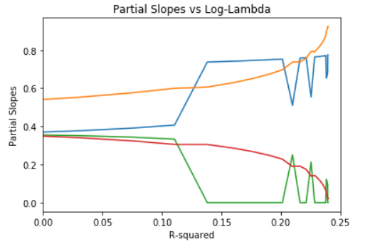 Notice that the elastic net model combines some of the behaviors of both L2 and L1 regularization.
Conclusion
In this article and last week's I looked at 3 methods as a solution to the problem of overfitting models:
- Stepwise Regression to eliminate features one at a time
- Singular Value Decomposition to find meaningful features
- Lasso, Ridge, and ElasticNet Regularization to stabilize over-parameterized models
Important terms include:
- AIC - the model log-likelihood adjusted for the number of model parameters
- Deviance - a measure of the relative likelihood of the model (a generalization of variance)
- SVD - Singular Value Decomposition describes a matrix as a linear combination of a series of vectors U, V, D
- Singular values s - the diagonal matrix of singular values used as a scaling term
- Lambda - a small bias term added to singular values to stabilize the inverse singular value matrix
- PCA - Principal Component Analysis to determine what new features can be made from linear combinations that are independent of each other by using functions and the SVD
- PCR - Principal Component Regression uses the PCA to perform a "regularized" regression
- L1 regularization - LASSO regularization using the "Manhattan" norm
- L2 Norm regularization - Ridge regularization limiting the "Euclidean" norm of values of the model coefficient vector
- ElasticNet algorithm - a weighted combination of L1 and L2 regularization
And I briefly reviewed linear algebra operations:
- Adding vectors and matrices
- Multiplying vectors and matrices
- Transposing matrices with
np.transpose
- Dot product or scalar product or inner product with
np.dot
- L2 norm of a vector
- Identity matrix with
np.eye
- Inverse of a matrix with
np.linalg.inv
- Singular value decomposition with
np.linalg.svd
- Creating a diagonal matrix with
np.diag
Up to now, I have been working strictly with linear regression models. Next, I will look at a widely used variation on the linear model know as logistic regression!
Find me on Linkedin
Physicist cum Data Scientist- Available for new opportunity | SaaS | Sports | Start-ups | Scale-ups
Register Now to Continue Reading
Unlock Towards Data Science with a Free Account
All articles on Towards Data Science are available to registered users. Create a free account today to access this article and thousands more.
Register for freeSign in to your account
 Written By
See all from James Andrew Godwin
Data ScienceMachine LearningPythonRegression AnalysisTowards Data Science
Share This Article
Towards Data Science is a community publication. Submit your insights to reach our global audience and earn through the TDS Author Payment Program.
Write for TDS
Related Articles
Data Science
How to calculate time-to-event probabilities and hazard rates for telecommunications subscribers.
Gustavo Santos
April 9, 202611 min read
Data Science
We discussed object detection on my previous article so this time around I'll be showing another example of how to identify objects...
Nico Aguila
January 30, 20213 min read
Machine Learning
Part 1 - Introduction
Patrick Altmeyer
October 24, 20225 min read
Artificial Intelligence
The unexpected running outcomes for Dictionary, Try Except and For-Loop
Christopher Tao
September 12, 20216 min read
Data Science
How to create an insightful graph
Elena Kosourova
March 27, 202113 min read
Machine Learning
Extract information from columns containing DateTime data. In the last two tutorials, we went from...
Ujjwal Dalmia
May 7, 20214 min read
Machine Learning
Processes and tools I used to deliver my first commercial machine learning model
Artur Lunardi Di Fante
December 15, 202112 min read
Artificial Intelligence
The most practical way to learn data science (Includes best-in-class references)
Sharan Kumar Ravindran
November 3, 202110 min read
Machine Learning
I'm hosting my Resnet-152 (152 layer CNN) model on AWS for pretty much free right now. Does it scale? What's the trade-offs?
Phil Whelan
March 17, 20218 min read
Your home for data science and AI. The world's leading publication for data science, data analytics, data engineering, machine learning, and artificial intelligence professionals.
Subscribe to Our NewsletterWrite For TDS•About•Advertise•Privacy Policy•Terms of Use
© Insight Media Group, LLC 2026•The New Stack•roadmap.sh•Creator Network
Recommended Articles
Close