 Image by Sascha Kirch.
保留正文与补采附件。源页面当前未重新核验;具体限制见交付清单。
Toggle SearchToggle Mobile Navigation Publish AI, ML & data-science insights to a global community of data professionals. Sign inSubmit an Article LatestEditor's PicksNewsletterShipAI
Write For TDS LinkedInXToggle Search Data Science
Part 4 - Towards Mamba State Space Models for Images, Videos and Time Series Sascha Kirch September 16, 202422 min read
Image by Sascha Kirch.
This is part 4 of my new multi-part series 🐍 Towards Mamba State Space Models for Images, Videos and Time Series. The field of computer vision has seen incredible advances in recent years. One of the key enablers for this development has been undoubtedly the introduction of the Transformer. While the Transformer has revolutionized natural language processing, it took us some years to transfer its capabilities to the vision domain. Probably the most prominent paper was the Vision Transformer (ViT), a model that is still used as the backbone in many of the modern architectures. It's again the Transformer's O(L²) complexity that limits its application as the image's resolution grows. Being equipped with the Mamba selective state space model, we are now able to let history repeat itself and transfer the success of SSMs from sequence data to non-sequence data: Images. ❗ Spoiler Alert: VisionMamba is 2.8x faster than DeiT and saves 86.8% GPU memory on high-resolution images (1248x1248) and in this article, you'll see how this is possible. Learn this step by step with the interactive AI and Data Scientist, Computer Science and Machine Learning roadmaps. Mamba State Space Models for Images, Videos and Time Series
Here Comes Mamba: The Selective State Space Model In part 3 we introduced Mamba as a new general-purpose architecture similar to the multi-head attention in the Transformer decoder. It incorporated selectivity into the state space model, transforming it into time-varying system. We gained a whole lot in terms of performance, but we lost the duality of the LTI system, where a recurrent system can be represented as a convolution. Hence Mamba was still fast at inference time but had to develop a new technique to enable fast and efficient training: the selective scan algorithm. This algorithm combined the associative parallel scan, kernel fusion, and the recomputation of gradients and carefully designed a CUDA implementation to be competitive with the Transformer in terms of performance and surpassing it in terms of speed.
It was a big day for deep learning, when back in 2017 A. Vaswani et .al. introduced the transformer architecture in Attention Is All You Need. This new model architecture did not only allow parallelizing the training process but also had basically no intrinsic bias and it seemed that the more data you throw at it the more performant it became.
Nearly everything related to sequences was done with the Transformer, resulting in a revolutionary time for NLP with prominent architectures like BERT, GPT or T5.
People desperately wanted to benefit from the Transformer's performance and its scaling laws for other data modalities beside text, but it wasn't until 2020, when another big paper by A. Dosovitskiy et. al. was released, finally applying Transformers on images: An Image is Worth 16x16 Words: Transformers for Image Recognition at Scale.
And here we are, in 2024, with a new promising architecture, namely Mamba, previously applied only to sequence-like data such as text and analog signals. What could be the next step? 🤔
Exactly, take the vision transformer paper and simply replace all occurrences of the word "Transformer" with the word "Mamba" and we are done!
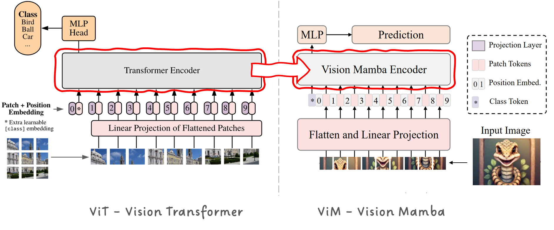 Figure 1: Comparing the ViT-Vision Transformer and the ViM-Vision Mamba models. Images taken from A. Dosovitskiy et. al. and L. Zhu et. al., annotated by Sascha Kirch.
Ok, that wasn't a good joke. Off course it is not that simple and there is much more to it.
❓ So, why would we like to replace the Transformer with Mamba in the first place when working with images?
What a strange thing to say... It is actually quite simple: The Transformer originates from natural language processing, where it was applied on sequences of words.
In ViT, to leverage the power of the Transformer for computer vision, an image was divided into 16x16 patches, and each patch was fed as an input into the Transformer. What previously have been words have now been individual image patches.
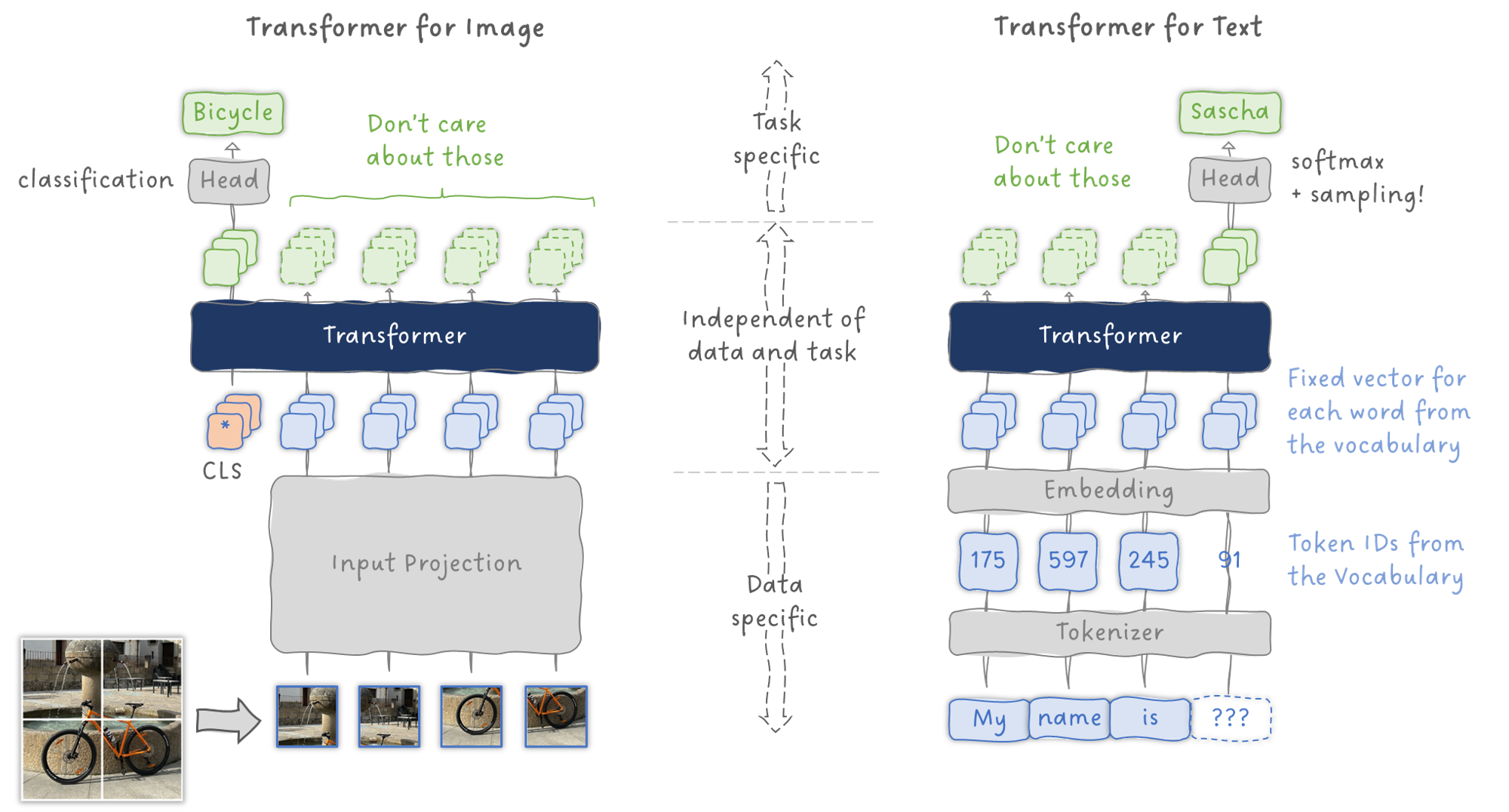 Figure 2: Comparing Transformer architectures for image classification and language modelling. Image by Sascha Kirch.
From this we can make quite an interesting observation: the Transformer block itself is independent from the data modality and from the actual task. It simply inputs a set of vectors and outputs a set of vectors. The way the data is prepared depends on the data modality at hand and the task we want to solve depends on what we are doing with those output vectors.
Coming back to ViT: We said the image was divided into 16x16 patches. The entire image though had a resolution of only 224x224 pixels during training (384 during fine-tuning), meaning each patch had a size of 14x14 pixels.
Even for that low resolution and that relatively large patch size, the compute requirements were already quite intense. The reason for that is that the work complexity of the Transformer scales quadratically with the sequence length L, often described as O(L²). This is the direct consequence of the attention mechanism that for each of the L tokens calculates how much it attends to the L other tokens. For 2D image patches that is even worse than for 1D sequence data. If you double the resolution (let's say 448x448) you end up with 4x more patches, i.e. 32x32=1024 instead of 16x16=256 as before. ❗ So, high resolution images are quite complicated to realize with a Transformer.
A looot of research has been focused on making the attention mechanism faster (e.g. Linformer and FlashAttention) or be able to process higher resolution images e.g. the Swin Transformer To gain some intuition on that, let's see how the number of image patches changes, if we keep the patch size constant and double image height and image width:
Figure 3: Increase in number of patches if doubling the image's resolution while keeping the patch's resolution fixed. Image by Sascha Kirch. And now lets see what happens if we keep the resolution of the image constant and simply decrease the size of the patch:
Figure 4: Increase in number of patches if keeping the image's resolution fixed while dividing the patch's resolution by 2. Image by Sascha Kirch. In both cases the number of patches increased by a factor of 4. Note that we only talked about the increase in the sequence length L. For the attention mechanism in the Transformer with its work complexity O(L²) that would mean a factor of 4 ²=16 more computations and memory. Also think about the performance impact of the patch size for a moment: the larger the patch, the more difficult it becomes to deal with smaller objects in the image. Decreasing the size of the patch has the same effect as increasing the resolution of the image and rapidly increases the number of patches. ❗ Small patches are also quite complicated to realize with the standard Transformer architecture. I guess by now you have a good intuition what would happen in an extreme case of taking a 4k image with its 3840x2160 pixels and using a patch size of 1x1. It would result in a sequence length of 8,294,400. Not saying it is a good idea to use such small patches, but you get the idea. 🤓 Get an email whenever Sascha Kirch publishes 🚀 _Get an email whenever Sascha Kirch publishes 🚀 Looking to learn more about deep learning or simply stay up to dat_e...medium.com
In previous parts of this series we introduced state space models and especially Mamba as an alternative to the Transformer architecture that promises better scaling laws with increased sequence lengths in terms of compute and memory requirements.
Towards Mamba State Space Models for Images, Videos and Time Series Up until now, Mamba has been designed for and applied on data of sequential nature like time signals or text. The challenge with images is, they are inherently non-sequential and contain spatial information such as local texture and global structure. Images are divided into patches and those are unrolled into a sequence, but there are many ways to unroll the image patches into a sequence. So, which one should we use?
Figure 5: Various ways to unroll a 2D grid of patches into a 1D sequence of patches. Image by Sascha Kirch. Recall that Mamba is a state space model. It recurrently updates its states from the previous state and new inputs. Hence, the order of inputs is quite important! In the attention-based Vision Transformer we didn't really need to care, because the attention mechanism has access to all other tokens of the sequence at any time. As long as we add the positional encoding to associate the patch with its spatial position we are fine. Let's consider the following example comparing state space models with attention-based model on which information of the input is available in their states at different positions:
Figure 6: State Space Model vs. Attention: How much information is contained in the model's state at different positions of the sequence. Image by Sascha Kirch. Note that in case of state space models, because of their recurrent nature, the state in the beginning of the sequence is less informed than the state at the end of the sequence. In the attention-based model, each state is equally informed by all other inputs of the sequence, regardless of their position. ❓ The question is, how do we add information of later patches in the sequence to earlier ones when using the SSM on images?
Well, one way to add information is to run the SSM twice: once forward and once backward. After that, we combine their respective results (Later in section 3 we'll see how this is done when diving into the architecture).
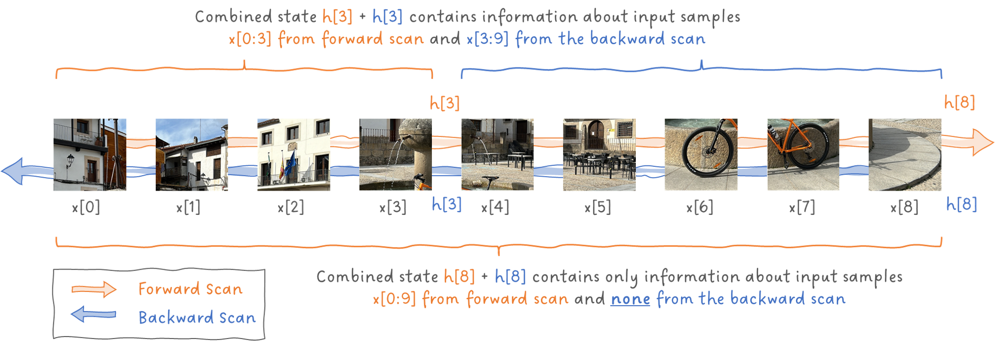 Figure 7: How a bidirectional scan of the sequence affects the information contained in the state of the SSM at different positions of the sequence. Image by Sascha Kirch.
We can make some interesting observations here:
Point 3 is quite interesting. Other papers like VMamba (parallel work similar to VisionMamba, released 1 day later) and MambaMixer (more details in part 6 of this series) add even more scanning directions (i.e. 4 as defined by the cross-scan) and have a slightly different architecture. Still, multiple SSMs are used for multiple scans.
That's an interesting but also difficult question to answer. Actually, some work focus on exactly that: showing that in some cases Mamba's selectivity is basically the same as attention. There is The Hidden Attention of Mamba Models and also Mamba-2 (what we will dive into in part 7 of this series).
After all, both models aim to find areas to focus on and areas to ignore in the data provided.
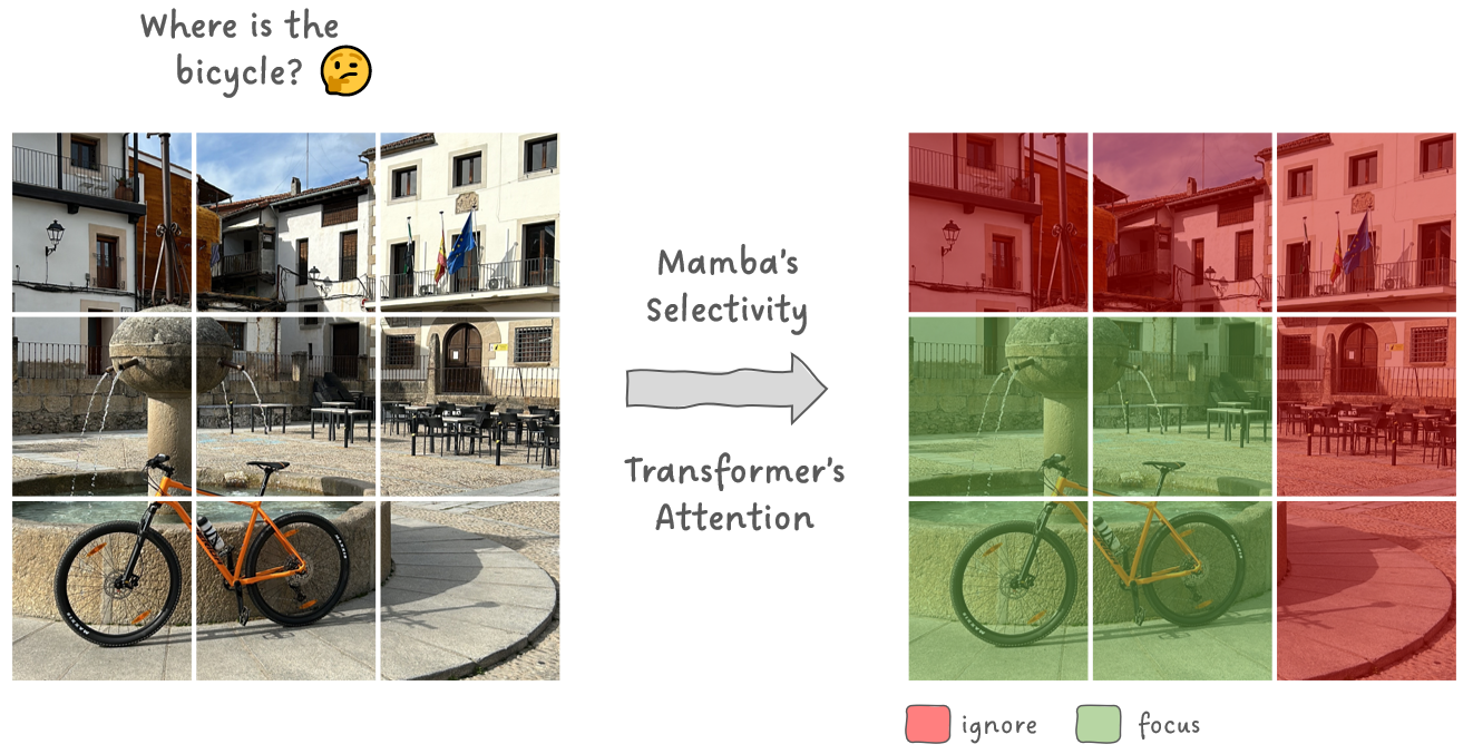 Figure 8: Selectivity and Attention on images. Image by Sascha Kirch.
The restrictions mentioned in most papers when drawing the connection between selectivity and attention is that SSMs behaves like causal attention such as in autoregressive sampling. In other words, we can only attend to past samples in the sequence since future samples are masked in the attention mask. Suddenly this duality feels slightly more natural, right? The difference between both methods is, that SSMs have a compressed state that represents the past and attention is not compressing its state at all having access to all samples at any time.
While the Transformer decoder is usually used as an autoregressive model when generating new text in an NLP task, for images we do not enforce these same restrictions and neither do we do it in a Transformer Encoder. The Transformer can attend to any patch at any time. We gain a lot by using SSMs on images (especially speed and memory consumption), but still intuitively it feels like it should not be as performant as attention, right?
In Fact, as we will see in section 3.2 when aiming to find the best bidirectional design, we'll see the importance of the joint forward and backward scan pattern for Vision Mamba's performance. So, apparently, there is no need to let everything attend to everything like the Transformer does, at least not in the presented tasks of object detection and image segmentation.
Equipped with some intuition on how Mamba could be a good fit for image data, let's review Vision Mamba's architecture:
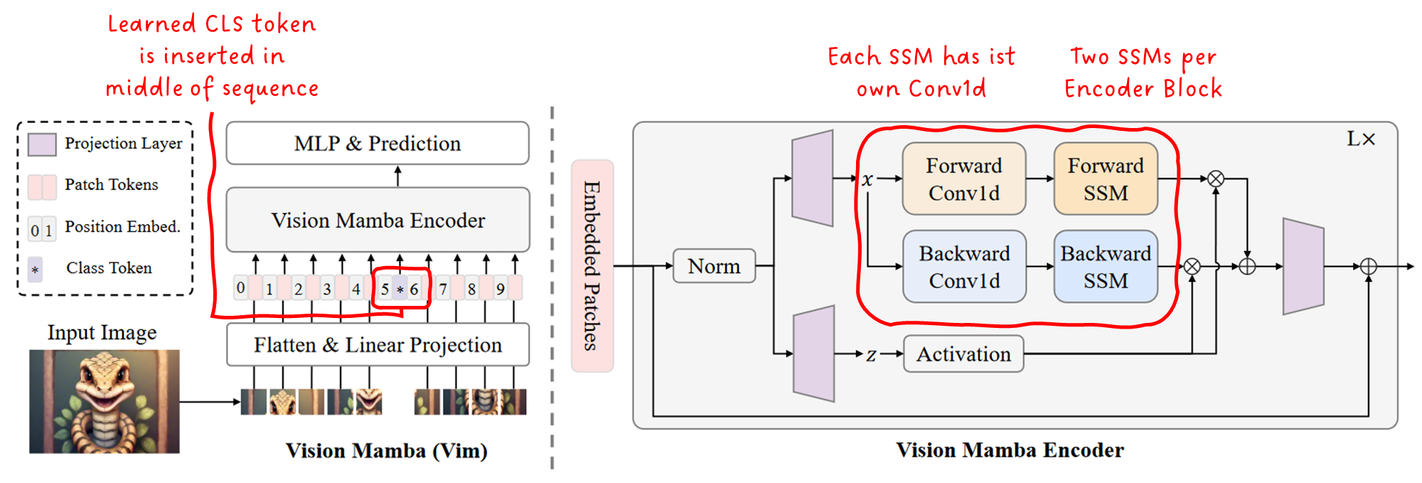 Figure 9: Top-Level architecture of Vision Mamba (Vim). Image by L. Zhu et.al., annotated by Sascha Kirch.
Compared to the ViT, Vision Mamba has two obvious differences: We have a Mamba encoder block instead of a Transformer encoder block and we insert the CLS token in the middle of the sequence rather than at the beginning.
On arxiv you'll find two versions of Vision Mamba: v1 and [v2](https://arxiv.org/abs/2401.09417v2). In v2 they mainly clarified the position of the CLS token, added a fine-tuning procedure for image classification, updated the images and added an extra ablation study concerned with different positions of the CLS token.
Having seen the top-level illustration of the architecture, let's zoom in to better understand what happens inside the encoder block.
Note that the names of dimensions and names for the modules are the same as in the official code implementation of the Vision Mamba Model to better understand how it can be configured and what is happening.
Figure 10: Detailed block diagram of the Mamba-Block used in Vision Mamba. In this example: L=4, d_model=3, expand=2, d_inner=6. Image by Sascha Kirch. There is a lot going here so let us go through it step by step. Let's start with the inputs and outputs. Each block gets the
hidden_statesand theresidualsfrom the previous layer as an input. Those are added in the beginning of the encoder, not at the end like shown in the top-level image. Further, they added a drop path regularization that occasionally drops the entirehidden_states. The block outputs the newhidden_statesandresidualto the next block. Notice that input and output have the same tensor dimensions. Continuing with the main block and just like in the Mamba block, we first normalize the input using RMS layer normalization and then linearly project it fromd_modeldimensions into2*d_innerdimensions, whered_inneris defined asexpand*d_model. Inside the codeexpanddefaults to 2. This output ofin_projis then split into 2 different paths, both of which are now of dimension[L, d_inner]. While one path is used as a skip connection, the other path is split again and fed into two independent SSMs , both with their own set of parameters, their own 1D convolution and their own states. Unlike indicated in the top-level architecture, these are not forward and backward SSMs, but rather two SSMs run forward, but the backward path simply flips the sequence. After the Selective SSM blocks , the two paths are combined and projected back fromd_innertod_modelto form the final output. Paper Walkthroughs by Sascha Kirch
In their ablation studies, they experiment with 3 different choices of bidirectional layer design:
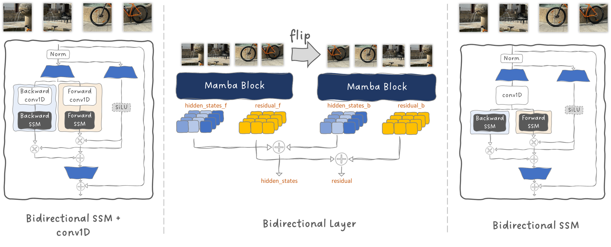 Figure 11: Various designs to incorporate bidirectionality into state space models. Image by Sascha Kirch.
Their final choice is the Bidirectional SSM + Conv1D , where each scan direction gets its own SSM (including the projections
x_proj and dt_proj) and their own Conv1D. Check-out their code.
The Bidirectional Layer , takes two simple Mamba Blocks, but one of those is input with the flipped input sequence. The resulting hidden_states and residuals are simply added together to form the final output. Check-out their code.
Finally, the Bidirectional SSM , adds a second SSM for the backward scan, BUT reuses the forward convolution and the input projections inside the SSM that construct matrices B and Δ. Hence only the state matrix A is learned. Check-out their code.
Here are the results of their ablation studies for image classification ImageNet and semantic segmentation on ADE20k.
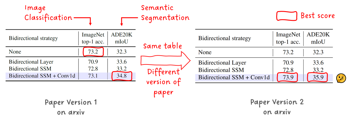 Figure 12: Ablation results of different bidirectional designs comparing version v1 and v2 of the arxiv paper. Tables by L. Zhu et.al., annotated by Sascha Kirch.
Interestingly those metrics changed between the different versions of the paper. It looks like they spent some extra effort to improve upon their previous results. Though, it is a bit suspicious that only the metrics for their proposed solution changed so let's hope it is no confirmation bias 🤭 In version 1 it looked like, no bidirectional scan is required for global image classification, but it becomes more important for dense prediction tasks like semantic segmentation.
After reading the Vision Mamba paper for the first time (and even after the 2nd and 3rd time 😅 ) I was left with 2 big question marks:
❓ So, why do we even need positional embeddings in the first place? This is what the creators of the Transformer said about that: "Since our model contains no recurrence and no convolution , in order for the model to make use of the order of the sequence, we must inject some information about the relative or absolute position of the tokens in the sequence." -A. Vaswani et. al., Attention is all you need. That's interesting, because Mamba is a selective SSM and its recurrency is one of its major motivations to use it. We update the state sequentially combining new inputs with the previous state so intuitively the model should know to which position the token belongs to. The authors of Vision Mamba don't go much into detail of why we need the position embeddings, but if you look carefully, you'll find two small hints: "[...] SSMs for data-dependent global visual context modeling and position embeddings for location-aware visual recognition . [...] the position embedding in Vim block provides the awareness for spatial information , which enables Vim to be more robust in dense prediction tasks." How I interpret this is, that the position embedding is rather to locate tokens in the spatial context than in the position of the sequence. As we learned earlier, a 2D image is a non-sequential data representation. While this kind of makes sense, we still have a recurrent SSM and if we feed the image patches every time in the same order, we should be able to infer the spatial location, right? At least that's what my gut tells me. ❗ My own speculative opinion on why it still might be a good idea to add position embeddings: (Let me know in the comments if you share this view or have an alternative intuition!)
❓ Why should we add the positional embedding in the middle?
First let's have a look on their ablation results and how the different strategies could be visualized:
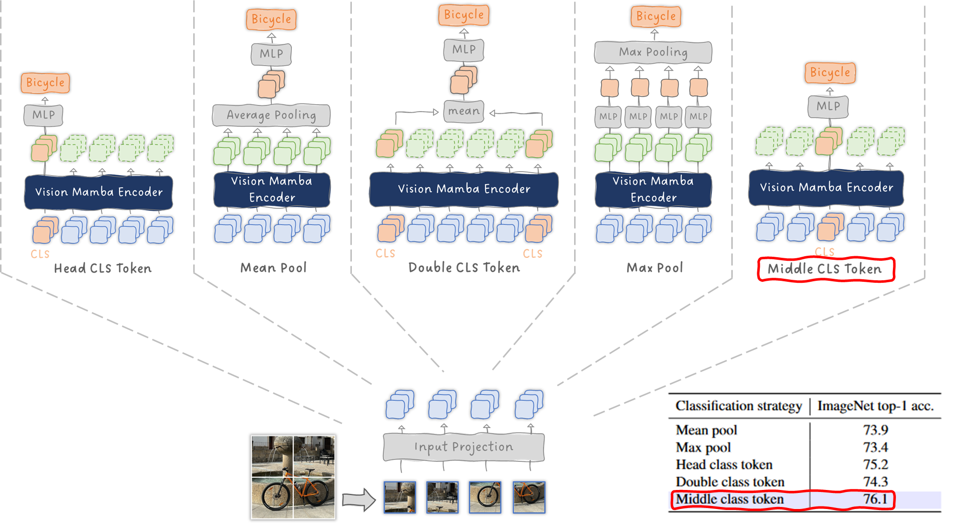 Figure 13: Comparing different classification strategies and CLS token positions. Table taken from L. Zhu et.al., image by Sascha Kirch.
What I find quite interesting is, why did they not test a with "Tail CLS Token" or simply take the output of the last token since in the recurrent update that would be constructed from the most informed state?
So, it feels kind of strange, that the best performing option is to use the middle cls token. The authors where not very specific on why they think this is the best option.
❗ So here is my own speculative opinion on that: (Let me know in the comments what you think could be an explanation!)
First, let us appreciate that adding a CLS token in general improves the classification performance, so let's forget about the mean pool and max pool configuration.
Further, remember that they implemented a forward and a backward SSM into their encoder blocks, so, at different positions of the sequence, each scan has seen different portions of the image.
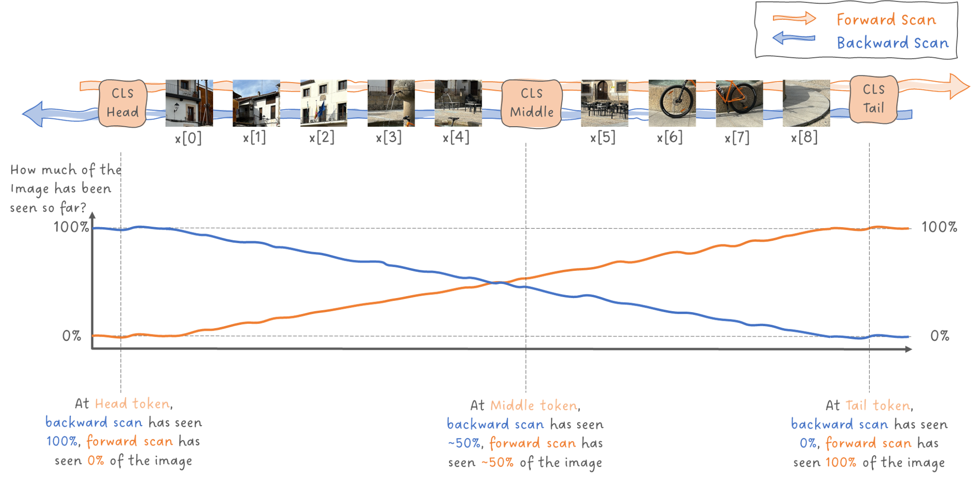 Figure 14: Relative amount of patches each scan has seen at various positions of the input sequence. Image by Sascha Kirch.
Having this in mind, let's go over the different CLS token types:
Head CLS Token - It has the 2nd highest score. I guess this comes from the fact, that the final state of the backward scan is at the head of the sequence, meaning it is the most informed state. The forward scan on the other hand, has seen no samples so far. The forward scan would be most informed at the tail of the sequence. So, I guess a head CLS token would have the similar performance as a tail CLS token (which they did not test). Both token types head and tail, have their main contribution either from the backward scan or the forward scan respectively.
Double CLS Token - It is slightly worse than the head CLS token. I guess this is again because for the outer tokens, either the forward or the backward scan dominates the prediction. Since the states are not coupled, but are independent from each other, they might not agree and have focused on different things in their selective state update.
Middle CLS Token - The best performing option. Notice that the middle of the sequence corresponds to the center patch of the image. Also, there is a thing called the photographer's bias , where in most photos the object of interest is placed in the center of the image. Since a SSM has a compressed state, it must decide what to keep and what to forget when updating its state. So, in my opinion one reason for the good performance of the middle CLS token could be combination of the photographer's bias together with the fact that the corresponding state for the center patch haven't had to forget prio information in favor of new inputs, yet.
As you might know, there are a lot of ways one could encode the position of a token and all those techniques come with different pros and cons. You could use absolute positions like an index or evaluating sinusoidal functions, you could use relative distances between the tokens, or something more sophisticated such as Rotary Positional Embeddings (RoPE), like it is used in modern LLMs like Meta's LLaMa or Google's PaLM. So, just for completeness, they don't mention it in the paper, but from their code we can see that they learn absolute positional embeddings.
Note: In the code of VisionMamba you'll find an implementation of Rotary Positional Embeddings (RoPE). Apparently none of their models activate those and they also don't mention it in the paper. So, either it was not working properly or it was so good they are currently writing on a new paper 😁
Let's briefly look on how Vision Mamba performs compared to its Transformer-based predecessor: DeiT. We are mainly concerned with two aspects: Its performance for various downstream tasks and the required resources in terms of inference speed and GPU memory footprint.
The paper presented us experiments for 4 different downstream tasks, namely:
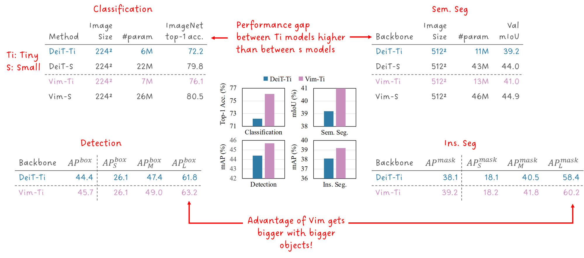 Figure 15: Performance comparision between VisionMAmba (ViM) and DeiT. Plot and values taken from L. Zhu et.al., illustrated by Sascha Kirch.
We can see that Vim performs especially well on large objects. The intuition is, that large objects occupy more space on the image hence appear in more image patchs, meaning the span a larger range in the input sequence.
To compare the resource needs of each of the model architectures, they performed batch inference on the vision backbones on a GPU with 80GB of memory.
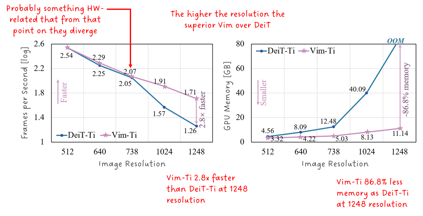 Figure 16: Comparing inference speed and memory needs for various image resolutions between VisionMAmba (ViM) and DeiT. Image by L. Zhu et.al., annotated by Sascha Kirch.
We see that due to the sub quadratic scaling of the Mamba architecture, especially high-resolution images benefit from the Vision Mamba architecture.
Interestingly, the inference speed is quite similar for resolutions up until 738. Probably because we have to move more data and need to perform more computations and from that point on we cannot use the HW resources as efficient as before (e.g. more memory reads, no coalesced memory accesses, exceeding size of shared memory and need to go to global memory, etc.), but that's just another of my hypothesis that might be wrong.
Vision Mamba applied Mamba-like state space models on images. The sub quadratic scaling law of Mamba-like state space models compared to their Transformer-based counter parts is especially well suited for dense-prediction tasks on high-resolution images. We have seen from the top-level architecture of Vision Mamba and Vision Transformer that they might appear to be quite similar. Their fundamental differences on how sequences are incorporated into their state representation, required us to revisit initial design choices of the Vision Transformer and we had to hypothesize why and how we can transfer them to Vision Mamba. We are now equipped with a model that can handle very long sequences efficiently and is capable to deal with non-sequential data such as images. ❓ And, what data modality deals with very long sequences of non-sequential data? Videos, exactly! So, that's what we will dive into next.
🤝 I'd like to thank you, t he readers of my stories, for your constant support, clapping f or my stories and, following m e to never miss any of my latest articles. It is you who motivates me to continue writing, dive deep into complex topics, and become a better engineer/researcher by writing about them. You are awesome!
VideoMamba - Understanding Videos 🔜 I am currently writing Part 5 of the series. I'll paste the link here once it is published! In Part 5 we will learn about deep learning for videos in general which we then us to motivate why Mamba-based models could be beneficial. Equipped with this intuition, we'll dive deeper into the VideoMamba model architecture and how it evolved from VisionMamba to deal with long range dependencies through time while still beeing able to detect short-term actions. We'll also see how VideoMamba can be combined with text resulting in a modern multi-modal model. Finally, we will close part 5 by comparing its performance with previous transformer-based and convolution based approaches.
Paper Walkthroughs by Sascha Kirch Mamba State Space Models for Images, Videos and Time Series
 Written By
See all from Sascha Kirch Deep DivesData ScienceMachine LearningMamba Image Video SignalProgramming Share This Article
Towards Data Science is a community publication. Submit your insights to reach our global audience and earn through the TDS Author Payment Program. Write for TDS

Data Science Rule-based Sentiment Analysis Using Python and R Paul Apivat January 29, 20219 min read

Machine Learning Social Media: The Challenge in Taking Action osintalex January 21, 20218 min read
Machine Learning Why you should be optimistic about the AI revolution Michael Malin August 24, 20216 min read

Artificial Intelligence In-database machine learning? It's easier than you think. Dario Radečić November 10, 20205 min read

Programming Python code to create folders and Word documents for research papers in biomedical sciences - all in one go with only two inputs Rodrigo M Carrillo Larco, MD, PhD December 8, 20246 min read
Machine Learning Step-by-step guide to continuous delivery of Custom Images in a Studio domain Sofian Hamiti May 16, 20215 min read
Machine Learning Explanation and Code Implementation Jeremy Zhang February 1, 20205 min read

Artificial Intelligence Real-world benchmarks for Llama-2 13B Het Trivedi August 8, 20237 min read

Artificial Intelligence Yes, hands-on examples in Python included. Dario Radečić December 8, 20204 min read
Your home for data science and AI. The world's leading publication for data science, data analytics, data engineering, machine learning, and artificial intelligence professionals. Subscribe to Our NewsletterWrite For TDS•About•Advertise•Privacy Policy•Terms of Use © Insight Media Group, LLC 2026•The New Stack•roadmap.sh•Creator Network
Close