保留正文与补采附件。源页面当前未重新核验;具体限制见交付清单。
 We value your privacy
We use cookies to enhance your browsing experience, serve personalised ads or content, and analyse our traffic. By clicking "Accept All", you consent to our use of cookies.
Customise Reject All Accept All
Customise Consent Preferences
 We use cookies to help you navigate efficiently and perform certain functions. You will find detailed information about all cookies under each consent category below.
The cookies that are categorised as "Necessary" are stored on your browser as they are essential for enabling the basic functionalities of the site. ... Show more
NecessaryAlways Active
Necessary cookies are required to enable the basic features of this site, such as providing secure log-in or adjusting your consent preferences. These cookies do not store any personally identifiable data.
-
Cookie
BCTempID
-
Duration
10 minutes
-
Description
No description available.
-
Cookie
__cf_bm
-
Duration
1 hour
-
Description
This cookie, set by Cloudflare, is used to support Cloudflare Bot Management.
-
Cookie
AWSALBCORS
-
Duration
7 days
-
Description
Amazon Web Services set this cookie for load balancing.
-
Cookie
_cfuvid
-
Duration
session
-
Description
Cloudflare sets this cookie to track users across sessions to optimize user experience by maintaining session consistency and providing personalized services
-
Cookie
li_gc
-
Duration
6 months
-
Description
Linkedin set this cookie for storing visitor's consent regarding using cookies for non-essential purposes.
-
Cookie
__hssrc
-
Duration
session
-
Description
This cookie is set by Hubspot whenever it changes the session cookie. The __hssrc cookie set to 1 indicates that the user has restarted the browser, and if the cookie does not exist, it is assumed to be a new session.
-
Cookie
__hssc
-
Duration
1 hour
-
Description
HubSpot sets this cookie to keep track of sessions and to determine if HubSpot should increment the session number and timestamps in the __hstc cookie.
-
Cookie
wpEmojiSettingsSupports
-
Duration
session
-
Description
WordPress sets this cookie when a user interacts with emojis on a WordPress site. It helps determine if the user's browser can display emojis properly.
-
Cookie
BCSessionID
-
Duration
1 year 1 month 4 days
-
Description
Blueconic sets this cookie as a unique identifier for the BlueConic profile.
-
Cookie
_octo
-
Duration
1 year
-
Description
No description available.
-
Cookie
logged_in
-
Duration
1 year
-
Description
No description available.
-
Cookie
__Secure-YEC
-
Duration
past
-
Description
YouTube sets this cookie to stores the user's video player preferences using embedded YouTube video
-
Cookie
__eoi
-
Duration
6 months
-
Description
Description is currently not available.
-
Cookie
AWSALBTGCORS
-
Duration
7 days
-
Description
No description available.
-
Cookie
login-status-p
-
Duration
past
-
Description
Description is currently not available.
-
Cookie
AWSALBTG
-
Duration
7 days
-
Description
No description available.
-
Cookie
csrf_token
-
Duration
session
-
Description
No description available.
-
Cookie
token_v2
-
Duration
1 day
-
Description
Description is currently not available.
-
Cookie
D
-
Duration
1 year
-
Description
Description is currently not available.
-
Cookie
PHPSESSID
-
Duration
session
-
Description
This cookie is native to PHP applications. The cookie stores and identifies a user's unique session ID to manage user sessions on the website. The cookie is a session cookie and will be deleted when all the browser windows are closed.
-
Cookie
VISITOR_PRIVACY_METADATA
-
Duration
6 months
-
Description
YouTube sets this cookie to store the user's cookie consent state for the current domain.
-
Cookie
cookietest
-
Duration
session
-
Description
The cookietest cookie is typically used to determine whether the user's browser accepts cookies, essential for website functionality and user experience.
-
Cookie
__Host-airtable-session
-
Duration
1 year
-
Description
This cookie is used to enable us to integrate the services of Airtable.
-
Cookie
__Host-airtable-session.sig
-
Duration
1 year
-
Description
This cookie is used to enable us to integrate the services of Airtable.
-
Cookie
m
-
Duration
1 year 1 month 4 days
-
Description
Stripe sets this cookie for fraud prevention purposes. It identifies the device used to access the website, allowing the website to be formatted accordingly.
-
Cookie
BIGipServer*
-
Duration
session
-
Description
Marketo sets this cookie to collect information about the user's online activity and build a profile about their interests to provide advertisements relevant to the user.
-
Cookie
__cfruid
-
Duration
session
-
Description
Cloudflare sets this cookie to identify trusted web traffic.
-
Cookie
_GRECAPTCHA
-
Duration
6 months
-
Description
Google Recaptcha service sets this cookie to identify bots to protect the website against malicious spam attacks.
-
Cookie
__Secure-YNID
-
Duration
6 months
-
Description
Google cookie used to protect user security and prevent fraud, especially during the login process.
-
Cookie
cookieyes-consent
-
Duration
1 year
-
Description
CookieYes sets this cookie to remember users' consent preferences so that their preferences are respected on subsequent visits to this site. It does not collect or store any personal information about the site visitors.
Functional
Functional cookies help perform certain functionalities like sharing the content of the website on social media platforms, collecting feedback, and other third-party features.
-
Cookie
lidc
-
Duration
1 day
-
Description
LinkedIn sets the lidc cookie to facilitate data center selection.
-
Cookie
brw
-
Duration
1 year
-
Description
No description available.
-
Cookie
brwConsent
-
Duration
5 minutes
-
Description
Description is currently not available.
-
Cookie
WMF-Uniq
-
Duration
1 year
-
Description
Description is currently not available.
-
Cookie
loom_anon_comment
-
Duration
1 year
-
Description
No description available.
-
Cookie
loom_referral_video
-
Duration
session
-
Description
Description is currently not available.
-
Cookie
VISITOR_INFO1_LIVE
-
Duration
6 months
-
Description
A cookie set by YouTube to measure bandwidth that determines whether the user gets the new or old player interface.
-
Cookie
yt-remote-connected-devices
-
Duration
Never Expires
-
Description
YouTube sets this cookie to store the user's video preferences using embedded YouTube videos.
-
Cookie
ytidb::LAST_RESULT_ENTRY_KEY
-
Duration
Never Expires
-
Description
The cookie ytidb::LAST_RESULT_ENTRY_KEY is used by YouTube to store the last search result entry that was clicked by the user. This information is used to improve the user experience by providing more relevant search results in the future.
-
Cookie
yt-remote-device-id
-
Duration
Never Expires
-
Description
YouTube sets this cookie to store the user's video preferences using embedded YouTube videos.
-
Cookie
yt-remote-session-name
-
Duration
session
-
Description
The yt-remote-session-name cookie is used by YouTube to store the user's video player preferences using embedded YouTube video.
-
Cookie
yt-remote-fast-check-period
-
Duration
session
-
Description
The yt-remote-fast-check-period cookie is used by YouTube to store the user's video player preferences for embedded YouTube videos.
-
Cookie
yt-remote-session-app
-
Duration
session
-
Description
The yt-remote-session-app cookie is used by YouTube to store user preferences and information about the interface of the embedded YouTube video player.
-
Cookie
yt-remote-cast-available
-
Duration
session
-
Description
The yt-remote-cast-available cookie is used to store the user's preferences regarding whether casting is available on their YouTube video player.
-
Cookie
yt-remote-cast-installed
-
Duration
session
-
Description
The yt-remote-cast-installed cookie is used to store the user's video player preferences using embedded YouTube video.
-
Cookie
cp_session
-
Duration
3 months
-
Description
Codepen sets this cookie for Help systems found in the website.
-
Cookie
loid
-
Duration
1 year 1 month 4 days
-
Description
This cookie is set by the Reddit. The cookie enables the sharing of content from the website onto the social media platform.
Analytics
Analytical cookies are used to understand how visitors interact with the website. These cookies help provide information on metrics such as the number of visitors, bounce rate, traffic source, etc.
-
Cookie
__hstc
-
Duration
6 months
-
Description
Hubspot set this main cookie for tracking visitors. It contains the domain, initial timestamp (first visit), last timestamp (last visit), current timestamp (this visit), and session number (increments for each subsequent session).
-
Cookie
hubspotutk
-
Duration
6 months
-
Description
HubSpot sets this cookie to keep track of the visitors to the website. This cookie is passed to HubSpot on form submission and used when deduplicating contacts.
-
Cookie
_ga
-
Duration
1 year 1 month 4 days
-
Description
Google Analytics sets this cookie to calculate visitor, session and campaign data and track site usage for the site's analytics report. The cookie stores information anonymously and assigns a randomly generated number to recognise unique visitors.
-
Cookie
ga*
-
Duration
1 year 1 month 4 days
-
Description
Google Analytics sets this cookie to store and count page views.
-
Cookie
__Host-psifi.analyticsTrace
-
Duration
6 hours
-
Description
Description is currently not available.
-
Cookie
__Host-psifi.analyticsTraceV2
-
Duration
6 hours
-
Description
Description is currently not available.
-
Cookie
_gh_sess
-
Duration
session
-
Description
GitHub sets this cookie for temporary application and framework state between pages like what step the user is on in a multiple step form.
-
Cookie
YSC
-
Duration
session
-
Description
YSC cookie is set by Youtube and is used to track the views of embedded videos on Youtube pages.
-
Cookie
ajs_anonymous_id
-
Duration
1 year
-
Description
This cookie is set by Segment to count the number of people who visit a certain site by tracking if they have visited before.
-
Cookie
vuid
-
Duration
1 year 1 month 4 days
-
Description
Vimeo installs this cookie to collect tracking information by setting a unique ID to embed videos on the website.
Performance
Performance cookies are used to understand and analyse the key performance indexes of the website which helps in delivering a better user experience for the visitors.
-
Cookie
AWSALB
-
Duration
7 days
-
Description
AWSALB is an application load balancer cookie set by Amazon Web Services to map the session to the target.
-
Cookie
acq
-
Duration
past
-
Description
Description is currently not available.
-
Cookie
acq.sig
-
Duration
past
-
Description
Description is currently not available.
-
Cookie
ptc
-
Duration
2 years
-
Description
No description available.
Advertisement
Advertisement cookies are used to provide visitors with customised advertisements based on the pages you visited previously and to analyse the effectiveness of the ad campaigns.
-
Cookie
muc_ads
-
Duration
1 year 1 month 4 days
-
Description
Twitter sets this cookie to collect user behaviour and interaction data to optimize the website.
-
Cookie
guest_id_marketing
-
Duration
1 year 1 month 4 days
-
Description
Twitter sets this cookie to identify and track the website visitor.
-
Cookie
guest_id_ads
-
Duration
1 year 1 month 4 days
-
Description
Twitter sets this cookie to identify and track the website visitor.
-
Cookie
personalization_id
-
Duration
1 year 1 month 4 days
-
Description
Twitter sets this cookie to integrate and share features for social media and also store information about how the user uses the website, for tracking and targeting.
-
Cookie
guest_id
-
Duration
1 year 1 month 4 days
-
Description
Twitter sets this cookie to identify and track the website visitor. It registers if a user is signed in to the Twitter platform and collects information about ad preferences.
-
Cookie
bcookie
-
Duration
1 year
-
Description
LinkedIn sets this cookie from LinkedIn share buttons and ad tags to recognize browser IDs.
-
Cookie
__Secure-ROLLOUT_TOKEN
-
Duration
6 months
-
Description
YouTube sets this cookie to manage feature rollout and experimentation. It helps Google control which new features or interface changes are shown to users as part of testing and staged rollouts, ensuring consistent experience for a given user during an experiment.
-
Cookie
yt.innertube::nextId
-
Duration
Never Expires
-
Description
YouTube sets this cookie to register a unique ID to store data on what videos from YouTube the user has seen.
-
Cookie
yt.innertube::requests
-
Duration
Never Expires
-
Description
YouTube sets this cookie to register a unique ID to store data on what videos from YouTube the user has seen.
-
Cookie
session_tracker
-
Duration
session
-
Description
This cookie is set by the Reddit. This cookie is used to identify trusted web traffic. It also helps in adverstising on the website.
-
Cookie
edgebucket
-
Duration
session
-
Description
Reddit sets this cookie to save the information about a log-on Reddit user, for the purpose of advertisement recommendations and updating the content.
-
Cookie
did
-
Duration
1 year
-
Description
Arbor sets this cookie to show targeted ads to site visitors.This cookie expires after 2 months or 1 year.
Uncategorised
Other uncategorised cookies are those that are being analysed and have not been classified into a category as yet.
No cookies to display.
Reject All Save My Preferences Accept All
Toggle SearchToggle Mobile Navigation
Publish AI, ML & data-science insights to a global community of data professionals.
Sign inSubmit an Article
LatestEditor's PicksNewsletterShipAI
Write For TDS
LinkedInXToggle Search
Deep Learning
Policy Gradient Methods in Reinforcement Learning
Teaching a Car to Cross a Mountain using Policy Gradient Methods in Python: A Mathematical Deep Dive into Reinforcement Learning
Cristian Leo
May 29, 202428 min read
Teaching a car to cross a mountain using policy gradient methods in Python: A mathematical deep dive into reinforcement learning
 Image generated by DALL-E
Imagine you are trying to teach a dog to fetch a ball. At first, the dog has no idea what to do when you throw the ball. It might run in different directions, ignore the ball, or do something completely unrelated. Your goal is to teach the dog the best way to fetch the ball and bring it back to you.
Each time the dog does something, you either reward it with a treat or do nothing. If the dog runs toward the ball, you give it a treat. If it does something else, you don't. This set of guidelines or strategies that the dog follows to decide what to do is called a policy. Initially, these guidelines are random, but with training, they become more focused on fetching the ball.
Over time, the dog learns that running towards the ball results in treats. It starts to follow this strategy more often because it leads to rewards. This is essentially how Policy Gradient Methods work. In this article, we will explore their mechanisms and math, and we will use the OpenAI Gym to train a car to drive across mountains. Let's get started!
Learn this step by step with the interactive Machine Learning roadmap.
Index
1: Introduction to Policy Gradient Optimization ∘ 1.1: What is Policy Gradient? 2: The Anatomy of Policy Gradient Methods ∘ 2.1: Policy Representations ∘ 2.2: Objective Functions 3: Key Components of Policy Gradient Optimization ∘ 3.1: The Policy Network ∘ 3.2: The Reward Function ∘ 3.3: Gradient Estimation 4: Implementing a Policy Gradient Method from Scratch ∘ 4.1: Setting Up the Environment and Hyperparameters ∘ 4.2: Defining the Policy Network ∘ 4.3: Implementing the REINFORCE Algorithm ∘ 4.4: Optimizing Hyperparameters with Optuna ∘ 4.5: Running the Training Process 5: Conclusion References
1: Introduction to Policy Gradient Optimization
In reinforcement learning, the agent (like the dog) learns to perform actions to achieve the best outcomes (like fetching the ball for treats). Policy gradient optimization is about adjusting the guidelines (policy) the agent follows so that it can maximize its rewards over time.
1.1: What is Policy Gradient?
Unlike value-based methods like Q-learning, which estimate the value of actions in specific states, policy gradient methods adjust the policy's parameters to maximize the expected cumulative reward.
In reinforcement learning, a policy defines an agent's behavior by specifying the probability distribution over actions given by a state. Mathematically, a policy π is represented as π(a|s; θ), where "a" is the action, "s" is the state, and "θ" are the policy parameters.
The goal of policy gradient methods is to find the optimal policy parameters (θ*) that maximize the expected return J(θ), which is the expected cumulative reward the agent receives from interacting with the environment. This objective can be expressed as:
 Policy Gradient Objective Function - Image by Author
where "γ" is the discount factor, and "r_t" is the reward at time step "t".
To achieve this, policy gradient methods use the gradient ascent algorithm. The parameters "θ" are updated in the direction of the gradient of the expected return with respect to the policy parameters. The update rule can be written as:
 Policy Gradient Update Formula - Image by Author
where "α" is the learning rate, and ∇θ J(θ) is the gradient of the expected return with respect to the policy parameters.
The gradient ∇θ J(θ) is estimated using samples from the environment. One popular method for this is the REINFORCE algorithm, which uses the following gradient estimate:
 REINFORCE Formula - Image by Author
where "R" is the cumulative reward obtained from the sampled trajectory. This estimate leverages the log-likelihood trick to compute the gradient efficiently.
2: The Anatomy of Policy Gradient Methods
2.1: Policy Representations
The policy is the core component that determines the agent's behavior by mapping states to actions. The way this mapping is structured is called policy representation. There are several ways to represent policies, each with its advantages and trade-offs. Let's explore some common policy representations used in policy gradient methods.
2.1.1: Parametric Policies Parametric policies use a set of parameters, like the weights and biases of a neural network, to define the policy. Think of it like baking a cake: the recipe (policy) tells you the quantities (parameters) of each ingredient (weights and biases) you need. The policy is often modeled as a probability distribution over actions given a state, and the neural network helps determine this distribution.
Discrete Actions For environments with discrete action spaces, the policy can be represented as a categorical distribution. Imagine you're at a restaurant choosing a meal from a menu. The neural network outputs a probability for each possible dish, and you select one based on these probabilities. The softmax function converts the output into a probability distribution over actions, similar to how you weigh your options and pick one.
 Policy for discrete action spaces - Image by Author
Here, f(s ;θ) is the output of the neural network, and the softmax function converts the output into a probability distribution over actions.
Continuous Actions For environments with continuous action spaces, the policy is often represented as a Gaussian distribution. Picture adjusting the volume on a stereo: the neural network outputs the mean (desired volume) and standard deviation (how much you might adjust it up or down). The agent samples an action from this distribution, like finding the right volume level by slightly adjusting the knob around the desired setting.
 Policy for continuous action spaces - Image by Author
Here, μ(s ;θ) and σ(s ;θ) are the mean and standard deviation produced by the neural network for a given state s.
2.1.2: Non-Parametric Policies Non-parametric policies don't rely on a fixed set of parameters to define the policy. Instead, they use techniques like nearest neighbor or kernel-based methods. This is like having a flexible recipe book where you choose the best recipe based on what's in your pantry. These methods are less common in deep reinforcement learning but can be useful when flexibility and adaptability are needed.
2.1.3: Deterministic Policies While policy gradient methods are typically associated with stochastic policies, deterministic policies can also be used, especially in continuous action spaces. Deterministic policies directly map states to actions without introducing randomness in the action selection process.
The Deterministic Policy Gradient (DPG) algorithm optimizes deterministic policies by adjusting the policy parameters to maximize the expected return. The policy is represented as a deterministic function μ(s ;θ), and the gradient of the expected return is computed with respect to the policy parameters.
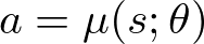 Deterministic Policy Formula - Image by Author
2.1.4: Hybrid Policies Hybrid policies combine elements of both parametric and non-parametric approaches. For example, a policy might use a neural network to parameterize a mixture of Gaussians, where the network outputs the parameters of multiple Gaussian distributions, and the final policy is a weighted sum of these distributions. Hybrid policies can provide additional flexibility and expressiveness in modeling complex behaviors.
2.2: Objective Functions
The objective function in policy gradient methods defines what the agent is trying to optimize. It measures how well a policy performs and guides the learning process by setting the criteria for updating policy parameters. In these methods, the goal is to maximize the expected cumulative reward. Let's explore different types of objective functions.
Expected Return The most basic objective function in policy gradient methods is the expected return. This represents the total expected reward an agent gets when following a policy, denoted as 𝜋, which is parameterized by 𝜃. The aim is to adjust the policy parameters 𝜃 to maximize this expected return.
Expected Return Formula - Image by Author
where:
- J(θ): The expected return as a function of the policy parameters θ.
- E__πθ_ : The expectation over the distribution of trajectories generated by the policy _π θ . This means we are averaging over all possible sequences of states and actions that the agent might encounter while following the policy _π θ .
- ∑ t =0: A sum over all time steps t from the start t =0 to the end t =T of the episode. This sum captures the cumulative reward.
- _γ t : The discount factor raised to the power of t. The discount factor γ ∈[0,1) determines how much future rewards are worth compared to immediate rewards. A smaller γ values immediate rewards more, while a γ closer to 1 values future rewards more.
- _r t : The reward received at time step t.
Log-Likelihood Objective To make optimization easier, the expected return can be expressed in terms of the policy's log-likelihood. This is done using the REINFORCE algorithm, where the objective function is:
 Log-Likelihood Formula - Image by Author
Here, log _π θ (a ∣ s) is the log-likelihood of taking action a in state s under the policy _π θ , and R is the cumulative reward obtained from the sampled trajectory. This formulation allows us to compute the gradient of the expected return concerning the policy parameters, which can then be used to update the policy via gradient ascent.
3: Key Components of Policy Gradient Optimization
3.1: The Policy Network
The policy network is the cornerstone of policy gradient methods, as it defines the agent's behavior by mapping states to actions. The design and implementation of the policy network are critical to the success of policy gradient optimization.
3.1.1: Network Architecture The architecture of the policy network plays a significant role in determining its ability to learn complex behaviors. Common architectures include:
Feedforward Neural Networks Feedforward Neural Networks are the simplest form of neural networks. They consist of multiple layers of neurons, where each layer is connected only to the next layer, with no loops or cycles. These networks are straightforward to implement and are effective for many tasks.
In the example below, we define a simple feedforward neural network in PyTorch. The network has three fully connected (or linear) layers. The first layer takes the input and maps it to 128 neurons. The second layer also has 128 neurons, and the third layer maps these to the output dimension, which represents the number of possible actions.
python
import torch
import torch.nn as nn
import torch.nn.functional as F

class PolicyNetwork(nn.Module):
    def __init__(self, input_dim, output_dim):
        super(PolicyNetwork, self).__init__()
        # Define the layers
        self.fc1 = nn.Linear(input_dim, 128)
        self.fc2 = nn.Linear(128, 128)
        self.fc3 = nn.Linear(128, output_dim)

    def forward(self, x):
        # Pass input through the layers with ReLU activation
        x = F.relu(self.fc1(x))
        x = F.relu(self.fc2(x))
        # Output layer with softmax to get probabilities
        x = F.softmax(self.fc3(x), dim=-1)
        return x
Here, the __init__ method initializes the network's layers. nn.Linear creates a fully connected layer.
The forward method defines the forward pass. It takes an input x, passes it through each layer, applies the ReLU activation function to introduce non-linearity, and finally uses a softmax function on the output layer to convert the outputs into probabilities.
If you want to learn more about this type of NN, here's an article for you:
The Math Behind Neural Networks
Recurrent Neural Networks (RNNs) Recurrent Neural Networks are designed to handle sequential data, making them ideal for environments where the agent needs to remember past states to make informed decisions. They have an internal memory that captures information about the sequence of states and actions.
In the following example, we use an LSTM (Long Short-Term Memory) network, a type of RNN, to create a policy network. The LSTM processes the input sequence and maintains a hidden state, which helps the network remember information over long sequences.
python
import torch
import torch.nn as nn
import torch.nn.functional as F

class RNNPolicyNetwork(nn.Module):
    def __init__(self, input_dim, output_dim):
        super(RNNPolicyNetwork, self).__init__()
        # Define an LSTM layer
        self.rnn = nn.LSTM(input_dim, 128, batch_first=True)
        self.fc = nn.Linear(128, output_dim)

    def forward(self, x, hx):
        # Pass input through the LSTM layer
        x, hx = self.rnn(x, hx)
        # Use the output from the last time step
        x = F.softmax(self.fc(x[:, -1, :]), dim=-1)
        return x, hx
The __init__ method initializes the LSTM layer and a fully connected layer.
The forward method processes the input sequence x and the hidden state hx through the LSTM. It uses the output from the last time step to make the final decision. The hidden state hx is updated and carried forward.
We covered extensively RNNs in this article:
The Math Behind Recurrent Neural Networks
You can also find an article specific to LSTMs here:
The Math Behind LSTM
Convolutional Neural Networks (CNNs) Convolutional Neural Networks are particularly effective for tasks involving spatially structured data, such as images. They use convolutional layers to automatically and adaptively learn spatial hierarchies of features from input data.
In this example, we define a CNN policy network. The network uses three convolutional layers to extract features from the input image and then passes these features through two fully connected layers to produce the output.
python
import torch
import torch.nn as nn
import torch.nn.functional as F

class CNNPolicyNetwork(nn.Module):
    def __init__(self, input_channels, output_dim):
        super(CNNPolicyNetwork, self).__init__()
        # Define convolutional layers
        self.conv1 = nn.Conv2d(input_channels, 32, kernel_size=8, stride=4)
        self.conv2 = nn.Conv2d(32, 64, kernel_size=4, stride=2)
        self.conv3 = nn.Conv2d(64, 64, kernel_size=3, stride=1)
        # Define fully connected layers
        self.fc1 = nn.Linear(64 * 7 * 7, 512)
        self.fc2 = nn.Linear(512, output_dim)

    def forward(self, x):
        # Pass input through convolutional layers with ReLU activation
        x = F.relu(self.conv1(x))
        x = F.relu(self.conv2(x))
        x = F.relu(self.conv3(x))
        # Flatten the tensor before passing to fully connected layers
        x = x.view(x.size(0), -1)
        x = F.relu(self.fc1(x))
        # Output layer with softmax to get probabilities
        x = F.softmax(self.fc2(x), dim=-1)
        return x
The __init__ method initializes three convolutional layers and two fully connected layers. Each convolutional layer applies a series of filters to the input data to extract different features.
The forward method passes the input through each convolutional layer with ReLU activation. After the convolutional layers, the data is flattened into a one-dimensional tensor using view. Finally, it passes through the fully connected layers, with the output layer using a softmax function to produce probabilities.
Here's an article to learn more about CNNs:
The Math Behind Convolutional Neural Networks
3.1.2: Output Layer The output layer of the policy network is designed to match the type of action space the agent operates in. This is crucial for the network to generate appropriate actions based on the learned policy.
Discrete Action Spaces For discrete action spaces, the output layer typically uses a softmax activation function. This function converts the raw outputs (logits) into a probability distribution over the possible discrete actions. Here's a simple implementation in PyTorch:
python
import torch.nn.functional as F

# Output for discrete actions
output = F.softmax(self.fc3(x), dim=-1)
This line of code applies the softmax function to the final fully connected layer's outputs (self.fc3(x)), producing a probability distribution where each value represents the probability of selecting a particular action.
Continuous Action Spaces In continuous action spaces, the output layer needs to produce probability distribution parameters over continuous actions. A common approach is to output a Gaussian distribution's mean and standard deviation. Here's how you can implement this:
python
import torch
import torch.nn as nn
import torch.nn.functional as F

class ContinuousPolicyNetwork(nn.Module):
    def __init__(self, input_dim, output_dim):
        super(ContinuousPolicyNetwork, self).__init__()
        self.fc1 = nn.Linear(input_dim, 128)
        self.fc2 = nn.Linear(128, 128)
        self.mean = nn.Linear(128, output_dim)
        self.log_std = nn.Linear(128, output_dim)

    def forward(self, x):
        x = F.relu(self.fc1(x))
        x = F.relu(self.fc2(x))
        mean = self.mean(x)
        log_std = self.log_std(x)
        std = torch.exp(log_std)
        return mean, std
In this code:
mean and log_std are the outputs of the final layers.log_std is transformed using torch.exp to ensure the standard deviation is positive.- The network outputs both
mean and std, which defines the Gaussian distribution for continuous actions.
3.1.3: Initialization Proper initialization of network parameters is essential for stable and efficient learning. Using good initialization techniques like Xavier (Glorot) initialization or He initialization helps maintain the variance of inputs and outputs across layers, preventing issues like vanishing or exploding gradients. Here's a function to initialize weights:
python
import torch.nn as nn

def init_weights(m):
    if isinstance(m, nn.Linear):
        nn.init.xavier_uniform_(m.weight)
        nn.init.constant_(m.bias, 0)

policy_network.apply(init_weights)
This function checks if a layer is a nn.Linear layer, if so it applies Xavier uniform initialization to its weights and sets the biases to zero.
3.1.4: Loss Function and Optimization In policy gradient methods, the loss function is derived from the objective function and usually involves the log-likelihood of actions weighted by rewards or advantages. The policy network is then optimized using gradient ascent or descent on this loss. Here's an example:
python
import torch.optim as optim

# Define the optimizer
optimizer = optim.Adam(policy_network.parameters(), lr=0.001)

# Training loop
for epoch in range(num_epochs):
    optimizer.zero_grad()
    loss = compute_policy_loss(policy_network, trajectories)
    loss.backward()
    optimizer.step()
Here:
optimizer.zero_grad() clears the gradients of all optimized parameters.compute_policy_loss is a hypothetical function that computes the loss based on policy gradients.loss.backward() computes the gradient of the loss for the network parameters.optimizer.step() updates the parameters based on the computed gradients.
3.2: The Reward Function
The reward function is a fundamental component in reinforcement learning, as it provides the feedback signal that drives the learning process. In policy gradient optimization, the reward function defines the goals of the agent and influences the policy updates by determining the rewards received from the environment. A well-designed reward function is crucial for guiding the agent towards desirable behaviors. Let's explore the key aspects of the reward function in policy gradient methods.
3.2.1: Designing the Reward Function Designing an effective reward function involves specifying the rewards in a way that aligns with the desired outcomes.
Sparse vs. Dense Rewards Sparse rewards are given infrequently, often only when the agent completes a task or reaches a goal. Dense rewards provide frequent feedback, offering rewards for intermediate steps towards the goal. Dense rewards can accelerate learning but may require careful tuning to avoid unintended behaviors.
python
def reward_function(state, action):
    if goal_reached(state):
        return 1.0  # Sparse reward
    return -0.01  # Dense reward for each time step
The function reward_function takes the current state and the action as inputs. It checks if the goal is reached using goal_reached(state). If true, it returns a reward of 1.0 (indicating success). If the goal is not reached, it returns a small negative reward (-0.01) for each time step, encouraging the agent to complete the task quickly.
Balancing Reward Components In tasks with multiple objectives, the reward function may need to balance different components. For example, in a robotic control task, the reward function might combine rewards for reaching a target, avoiding obstacles, and minimizing energy consumption.
python
 def reward_function(state, action):
    target_reward = compute_target_reward(state)
    obstacle_penalty = compute_obstacle_penalty(state)
    energy_penalty = compute_energy_penalty(action)
    return target_reward - obstacle_penalty - energy_penalty
This function balances multiple objectives:
compute_target_reward(state) provides a reward for reaching the target.compute_obstacle_penalty(state) adds a penalty for hitting obstacles.compute_energy_penalty(action) adds a penalty for using energy, encouraging efficient actions.
The total reward is a combination of these components, balancing the different objectives.
3.2.2: Discounted Rewards In policy gradient methods, future rewards are often discounted to reflect their present value. The discount factor (𝛾) determines how much future rewards are valued compared to immediate rewards. A discount factor close to 1 means the agent values future rewards almost as much as immediate rewards, while a lower discount factor places more emphasis on immediate rewards.
python
def compute_discounted_rewards(rewards, gamma):
    discounted_rewards = []
    cumulative_reward = 0
    for reward in reversed(rewards):
        cumulative_reward = reward + gamma * cumulative_reward
        discounted_rewards.insert(0, cumulative_reward)
    return discounted_rewards
The function compute_discounted_rewards calculates the discounted sum of future rewards.
gamma is the discount factor, determining how future rewards are valued compared to immediate rewards.
The function iterates over rewards in reverse order. For each reward, it updates the cumulative_reward by adding the current reward and the discounted future rewards. The cumulative reward is then inserted at the beginning of the discounted_rewards list.
This approach ensures that the agent evaluates the long-term value of actions, considering both immediate and future rewards
3.3: Gradient Estimation
Gradient estimation determines how we update the policy parameters to maximize the expected cumulative reward. The gradient of the objective function with respect to these parameters shows the direction to adjust them.
3.3.1: Monte Carlo Policy Gradient (REINFORCE) Imagine you're a coach training a player. After each game, you give feedback based on the game's result. The player uses this feedback to improve future performance. Similarly, the REINFORCE algorithm updates the policy based on the cumulative rewards from each trajectory.
The algorithm uses the log-likelihood trick to derive the gradient of the expected return. The gradient is computed using sampled trajectories from the policy, and the update rule is:
 REINFORCE Formula - Image by Author
where _R t is the cumulative reward from time step t to the end of the episode.
Here's a Python implementation:
python
def compute_policy_gradient(policy_network, trajectories, gamma=0.99):
    policy_gradients = []
    for trajectory in trajectories:
        states, actions, rewards = trajectory
        discounted_rewards = compute_discounted_rewards(rewards, gamma)
        for t, (state, action, reward) in enumerate(zip(states, actions, discounted_rewards)):
            state_tensor = torch.tensor(state, dtype=torch.float32)
            action_tensor = torch.tensor(action, dtype=torch.int64)
            reward_tensor = torch.tensor(reward, dtype=torch.float32)

            log_prob = torch.log(policy_network(state_tensor)[action_tensor])
            policy_gradients.append(-log_prob * reward_tensor)

    return torch.stack(policy_gradients).sum()
In this code, we iterate over trajectories, which are sequences of states, actions, and rewards. For each state-action pair, we compute the log probability of the action under the current policy and multiply it by the discounted reward. The negative sign ensures we are maximizing the reward.
4: Implementing a Policy Gradient Method from Scratch
Now it's finally time to get into action! In this section, we'll walk through implementing policy gradient methods in Python. By the end, you'll understand how to build and train a policy gradient model using the REINFORCE algorithm. We'll use the MountainCar-v0 environment from OpenAI Gym. The environment is free for commercial use. You can find more details about the license and usage rights on the OpenAI Gym GitHub page. The goal is to drive a car up a steep hill. The car can accelerate left, right, or not at all, and the objective is to reach the top of the hill.
You can find the full code here:
Reinforcement-Learning/4. Polict Gradient Methods/main.py at main ·...
4.1: Setting Up the Environment and Hyperparameters
First, we need to import the necessary libraries and set up our environment and hyperparameters.
python
import os
import pickle
import gym
from gym.wrappers.monitoring.video_recorder import VideoRecorder
import torch
import torch.nn as nn
import torch.optim as optim
import gc
import optuna

gc.enable()

# Configuration
TRAIN = True
FINETUNE = False
SAVE_MODEL = True
SAVE_VIDEO = False
RENDER_MODE = 'rgb_array'

# Hyperparameters
TRAINING_EPISODES = 1000
FINETUNE_TRIALS = 100

# Default hyperparameters if not fine-tuning
GAMMA = 0.99
LEARNING_RATE = 1e-3
Here, gc.enable() enables automatic garbage collection to manage memory efficiently during training.
TRAIN, FINETUNE, SAVE_MODEL, and SAVE_VIDEO control whether to train, fine-tune, save the model, and save videos, respectively. RENDER_MODE specifies the rendering mode for the environment.
TRAINING_EPISODES and FINETUNE_TRIALS define the number of episodes for training and fine-tuning.
GAMMA and LEARNING_RATE are set as default hyperparameters for the discount factor and learning rate.
4.2: Defining the Policy Network
Then, we create a neural network to represent the policy. The network will map states to action probabilities using a series of fully connected layers with ReLU activations.
python
class PolicyNetwork(nn.Module):
    def __init__(self, state_dim, action_dim, device=torch.device('cpu')):
        super(PolicyNetwork, self).__init__()
        self.fc1 = nn.Linear(state_dim, 128)
        self.fc2 = nn.Linear(128, 128)
        self.fc3 = nn.Linear(128, action_dim)
        self.device = device
        self.to(device)
__init__ method initializes the network's layers. It includes three fully connected layers:
self.fc1: Maps the input state dimension to 128 neurons.self.fc2: Maps 128 neurons to another 128 neurons.self.fc3: Maps 128 neurons to the action dimension.
self.device sets the device for computations (CPU or GPU). self.to(device) moves the model to the specified device.
python
    def forward(self, x):
        x = torch.relu(self.fc1(x))
        x = torch.relu(self.fc2(x))
        return torch.softmax(self.fc3(x), dim=-1)
The forward method defines how data flows through the network. x is passed through the layers with ReLU activation functions. The output layer uses a softmax function to convert outputs into probabilities.
4.3: Implementing the REINFORCE Algorithm
The REINFORCE algorithm updates the policy based on the rewards obtained from sampled trajectories.
python
class REINFORCE:
    def __init__(self, env, policy_network, optimizer, model_path='model/model.pth', gamma=0.99):
        self.env = env
        self.policy_network = policy_network
        self.optimizer = optimizer
        self.model_path = model_path
        self.gamma = gamma

        if os.path.exists(os.path.dirname(self.model_path)):
            if os.path.isfile(self.model_path):
                self.policy_network.load_state_dict(torch.load(self.model_path))
                print("Loaded model from disk")
        else:
            os.makedirs(os.path.dirname(self.model_path))

    def train(self, num_episodes, save_model=SAVE_MODEL, save_video=SAVE_VIDEO):
        total_rewards = []

        if save_video:
            self.video = VideoRecorder(self.env, f'{os.path.dirname(__file__)}/training.mp4', enabled=True)

        for episode in range(num_episodes):
            state, _ = self.env.reset()
            done = False
            total_reward = 0
            log_probs = []
            rewards = []

            while not done:
                if RENDER_MODE == 'human':
                    self.env.render()

                if save_video:
                    self.video.capture_frame()

                state = torch.FloatTensor(state).unsqueeze(0).to(device)
                action_probs = self.policy_network(state)
                action = torch.multinomial(action_probs, 1).item()
                log_prob = torch.log(action_probs.squeeze(0)[action])
                log_probs.append(log_prob)

                next_state, reward, done, _, _ = self.env.step(action)
                rewards.append(reward)
                state = next_state
                total_reward += reward

            total_rewards.append(total_reward)
            self.update_policy(log_probs, rewards)

            print(f"Episode {episode}, Total Reward: {total_reward}")

            if episode % 5 == 0 and episode > 0:
                print(f"Episode {episode}, Average Reward: {sum(total_rewards) / len(total_rewards)}")
                if save_model:
                    torch.save(self.policy_network.state_dict(), self.model_path)
                    print("Saved model to disk")

            del log_probs, rewards, state, action_probs, action
            gc.collect()

        if save_model:
            torch.save(self.policy_network.state_dict(), self.model_path)
            print("Saved model to disk")

        if save_video:
            self.video.close()

        self.env.close()
        return sum(total_rewards) / len(total_rewards)

    def update_policy(self, log_probs, rewards):
        discounted_rewards = []
        for t in range(len(rewards)):
            Gt = sum(self.gamma ** i * rewards[t + i] for i in range(len(rewards) - t))
            discounted_rewards.append(Gt)

        discounted_rewards = torch.FloatTensor(discounted_rewards).to(device)
        discounted_rewards = (discounted_rewards - discounted_rewards.mean()) / (discounted_rewards.std() + 1e-9)

        policy_loss = []
        for log_prob, Gt in zip(log_probs, discounted_rewards):
            policy_loss.append(-log_prob * Gt)

        self.optimizer.zero_grad()
        policy_loss = torch.stack(policy_loss).sum()
        policy_loss.backward()
        self.optimizer.step()
Class Initialization
python
    def __init__(self, env, policy_network, optimizer, model_path='model/model.pth', gamma=0.99):
        self.env = env
        self.policy_network = policy_network
        self.optimizer = optimizer
        self.model_path = model_path
        self.gamma = gamma
__init__ method initializes the environment, policy network, optimizer, and model path.
self.env: The environment object.self.policy_network: The policy network object.self.optimizer: The optimizer object.self.model_path: Path to save/load the model.self.gamma: Discount factor for future rewards.
python
        if os.path.exists(os.path.dirname(self.model_path)):
            if os.path.isfile(self.model_path):
                self.policy_network.load_state_dict(torch.load(self.model_path))
                print("Loaded model from disk")
        else:
            os.makedirs(os.path.dirname(self.model_path))
Checks if the model path exists and loads the model if it exists:
Train Method
python
def train(self, num_episodes, save_model=SAVE_MODEL, save_video=SAVE_VIDEO):
        total_rewards = []

        if save_video:
            self.video = VideoRecorder(self.env, f'{os.path.dirname(__file__)}/training.mp4', enabled=True)

        for episode in range(num_episodes):
            state, _ = self.env.reset()
            done = False
            total_reward = 0
            log_probs = []
            rewards = []

            while not done:
                if RENDER_MODE == 'human':
                    self.env.render()

                if save_video:
                    self.video.capture_frame()

                state = torch.FloatTensor(state).unsqueeze(0).to(device)
                action_probs = self.policy_network(state)
                action = torch.multinomial(action_probs, 1).item()
                log_prob = torch.log(action_probs.squeeze(0)[action])
                log_probs.append(log_prob)

                next_state, reward, done, _, _ = self.env.step(action)
                rewards.append(reward)
                state = next_state
                total_reward += reward

            total_rewards.append(total_reward)
            self.update_policy(log_probs, rewards)

            print(f"Episode {episode}, Total Reward: {total_reward}")

            if episode % 5 == 0 and episode > 0:
                print(f"Episode {episode}, Average Reward: {sum(total_rewards) / len(total_rewards)}")
                if save_model:
                    torch.save(self.policy_network.state_dict(), self.model_path)
                    print("Saved model to disk")

            del log_probs, rewards, state, action_probs, action
            gc.collect()

        if save_model:
            torch.save(self.policy_network.state_dict(), self.model_path)
            print("Saved model to disk")

        if save_video:
            self.video.close()

        self.env.close()
        return sum(total_rewards) / len(total_rewards)
The training method runs the training loop for a specified number of episodes. It initializes an empty list to store the total rewards for each episode total_rewards = []. This list will store the total rewards for each episode. It helps in tracking the performance of the agent over time.
python
if save_video:
        self.video = VideoRecorder(self.env, f'{os.path.dirname(__file__)}/training.mp4', enabled=True)
If save_video is enabled, initialize a VideoRecorder to record the training process.
python
for episode in range(num_episodes):
        state, _ = self.env.reset()
        done = False
        total_reward = 0
        log_probs = []
        rewards = []
The outer loop runs for num_episodes, representing the number of episodes to train the agent. state, _ = self.env.reset() resets the environment to the initial state for each new episode.
Here:
done = False: A flag to indicate if the episode is finished.total_reward = 0: Accumulates the total reward for the current episode.log_probs = []: List to store log probabilities of actions taken.rewards = []: List to store rewards received.
python
        while not done:
            if RENDER_MODE == 'human':
                self.env.render()

            if save_video:
                self.video.capture_frame()

            state = torch.FloatTensor(state).unsqueeze(0).to(device)
            action_probs = self.policy_network(state)
            action = torch.multinomial(action_probs, 1).item()
            log_prob = torch.log(action_probs.squeeze(0)[action])
            log_probs.append(log_prob)

            next_state, reward, done, _, _ = self.env.step(action)
            rewards.append(reward)
            state = next_state
            total_reward += reward
The inner loop continues until done is True, indicating the end of the episode.
Firstly, state = torch.FloatTensor(state).unsqueeze(0).to(device) converts the state to a PyTorch tensor and moves it to the specified device (CPU or GPU). action_probs = self.policy_network(state) uses the policy network to get the action probabilities for the current state. action = torch.multinomial(action_probs, 1).item() samples an action from the action probabilities. log_prob = torch.log(action_probs.squeeze(0)[action]) computes the log probability of the selected action.
Then, we append the log probability and reward to their respective lists: log_probs.append(log_prob) and rewards.append(reward).
Next, next_state, reward, done, _, _ = self.env.step(action) take the action in the environment and observe the next state, reward, and whether the episode is done.
Finally, we update the state and the total reward with:
state = next_state , which updates the current state to the next state.total_reward += reward , which accumulates the total reward for the current episode.
python
        total_rewards.append(total_reward)
        self.update_policy(log_probs, rewards)

        print(f"Episode {episode}, Total Reward: {total_reward}")

        if episode % 5 == 0 and episode > 0:
            print(f"Episode {episode}, Average Reward: {sum(total_rewards) / len(total_rewards)}")
            if save_model:
                torch.save(self.policy_network.state_dict(), self.model_path)
                print("Saved model to disk")

        del log_probs, rewards, state, action_probs, action
        gc.collect()
At the end of each episode, the total reward of the current episode is appended to the total_rewards list: total_rewards.append(total_reward). The policy is updated using the collected log probabilities and rewards: self.update_policy(log_probs, rewards).
Every 5 episodes, the average reward is printed, and the model is saved if save_model is enabled.
Lastly, the variables are deleted to free up memory, and garbage collection is performed: del log_probs, rewards, state, action_probs, action and gc.collect().
python
    if save_model:
        torch.save(self.policy_network.state_dict(), self.model_path)
        print("Saved model to disk")

    if save_video:
        self.video.close()

    self.env.close()
    return sum(total_rewards) / len(total_rewards)
At the end of the training, the model is saved after training if save_model is enabled. torch.save(self.policy_network.state_dict(), self.model_path) saves the model state to disk. Then, the average reward over all episodes is returned.
Update Policy Method The update_policy method is responsible for updating the policy network based on the rewards obtained during an episode. This is achieved using the REINFORCE algorithm, which involves calculating the discounted rewards, normalizing them, and then computing the policy loss to update the network parameters.
python
    def update_policy(self, log_probs, rewards):
        discounted_rewards = []
        for t in range(len(rewards)):
            Gt = sum(self.gamma ** i * rewards[t + i] for i in range(len(rewards) - t))
            discounted_rewards.append(Gt)

        discounted_rewards = torch.FloatTensor(discounted_rewards).to(device)
        discounted_rewards = (discounted_rewards - discounted_rewards.mean()) / (discounted_rewards.std() + 1e-9)

        policy_loss = []
        for log_prob, Gt in zip(log_probs, discounted_rewards):
            policy_loss.append(-log_prob * Gt)

        self.optimizer.zero_grad()
        policy_loss = torch.stack(policy_loss).sum()
        policy_loss.backward()
        self.optimizer.step()
discounted_rewards = [] initializes an empty list to store the discounted rewards for each time step.
The loop for t in range(len(rewards)) iterates over each time step t in the list of rewards. For each time step t, the discounted reward Gt is calculated using the formula:
 Discounted Rewards Formula - Image by Author
Here,
self.gamma is the discount factor, and rewards[t + i] are the rewards from the time step t to the end of the episode. The calculated discounted reward Gt is then appended to the discounted_rewards list: discounted_rewards.append(Gt).
python
discounted_rewards = torch.FloatTensor(discounted_rewards).to(device)
discounted_rewards = (discounted_rewards - discounted_rewards.mean()) / (discounted_rewards.std() + 1e-9)
The list of discounted rewards is converted to a PyTorch tensor and moved to the specified device (CPU or GPU) using discounted_rewards = torch.FloatTensor(discounted_rewards).to(device).
The discounted rewards are normalized to have zero mean and unit standard deviation using the formula:
 Discounted Rewards Normalization Formula - Image by Author
This normalization helps to stabilize training.
go
    policy_loss = []
    for log_prob, Gt in zip(log_probs, discounted_rewards):
        policy_loss.append(-log_prob * Gt)
policy_loss = [] initializes an empty list to store the policy loss for each time step. The loop for log_prob, Gt in zip(log_probs, discounted_rewards) iterates over each log probability and its corresponding discounted reward.
For each log probability log_prob and discounted reward Gt, the loss is calculated as -log_prob * Gt and appended to the policy_loss list: policy_loss.append(-log_prob * Gt).
python
    self.optimizer.zero_grad()
    policy_loss = torch.stack(policy_loss).sum()
    policy_loss.backward()
    self.optimizer.step()
The gradients are zeroed out before the backward pass using self.optimizer.zero_grad(). The list of policy losses is stacked into a single tensor and summed up using policy_loss = torch.stack(policy_loss).sum().
Then, the backward pass is performed to compute the gradients of the policy loss with respect to the network parameters using policy_loss.backward().
Lastly, the optimizer updates the network parameters based on the computed gradients using self.optimizer.step().
4.4: Optimizing Hyperparameters with Optuna
In this implementation, we use Optuna to find the best hyperparameters for our reinforcement learning model. Optuna is an automatic hyperparameter optimization framework designed to optimize machine learning models efficiently.
python
class Optimizer:
    def __init__(self, env, policy_network, model_path, params_path='params.pkl'):
        self.env = env
        self.policy_network = policy_network
        self.model_path = model_path
        self.params_path = params_path

    def objective(self, trial, n_episodes=100):
        lr = trial.suggest_loguniform('lr', 1e-5, 1e-1)
        gamma = trial.suggest_uniform('gamma', 0.9, 0.999)
        optimizer = optim.Adam(self.policy_network.parameters(), lr=lr)
        trainer = REINFORCE(self.env, self.policy_network, optimizer, self.model_path, gamma=gamma)
        reward = trainer.train(n_episodes, save_model=False, save_video=False)
        return reward

    def optimize(self, n_trials=100, save_params=True):
        if not TRAIN and os.path.isfile(self.params_path):
            with open(self.params_path, 'rb') as f:
                best_params = pickle.load(f)
            print("Loaded parameters from disk")
        elif not FINETUNE:
            best_params = {'lr': LEARNING_RATE, 'gamma': GAMMA}
            print(f"Using default parameters: {best_params}")
        else:
            print("Optimizing hyperparameters")
            study = optuna.create_study(direction='maximize')
            study.optimize(self.objective, n_trials=n_trials)
            best_params = study.best_params
            if save_params:
                with open(self.params_path, 'wb') as f:
                    pickle.dump(best_params, f)
                print("Saved parameters to disk")
        return best_params
Class Initialization The Optimizer class is designed to optimize the hyperparameters of the policy network. It takes the environment, policy network, model path, and parameters path as inputs.
ruby
class Optimizer:
    def __init__(self, env, policy_network, model_path, params_path='params.pkl'):
        self.env = env
        self.policy_network = policy_network
        self.model_path = model_path
        self.params_path = params_path
Here:
self.env is the environment object in which the agent operates.self.policy_network is the neural network model representing the policy.self.model_path is the path where the trained model will be saved or loaded from.self.params_path is the path where the best hyperparameters will be saved or loaded from.
Objective Method
The objective method defines the objective function for Optuna to optimize. It suggests hyperparameters for the learning rate and discount factor, trains the model with these parameters and returns the average reward.
python
    def objective(self, trial, n_episodes=100):
        lr = trial.suggest_loguniform('lr', 1e-5, 1e-1)
        gamma = trial.suggest_uniform('gamma', 0.9, 0.999)
        optimizer = optim.Adam(self.policy_network.parameters(), lr=lr)
        trainer = REINFORCE(self.env, self.policy_network, optimizer, self.model_path, gamma=gamma)
        reward = trainer.train(n_episodes, save_model=False, save_video=False)
        return reward
lr = trial.suggest_loguniform('lr', 1e-5, 1e-1) suggests a learning rate within the range [1e-5, 1e-1]. The loguniform distribution ensures that the learning rate is sampled on a logarithmic scale.
gamma = trial.suggest_uniform('gamma', 0.9, 0.999) suggests a discount factor within the range [0.9, 0.999].
optimizer = optim.Adam(self.policy_network.parameters(), lr=lr) initializes the Adam optimizer with the suggested learning rate.
trainer = REINFORCE(self.env, self.policy_network, optimizer, self.model_path, gamma=gamma) creates a REINFORCE trainer with the suggested hyperparameters.
reward = trainer.train(n_episodes, save_model=False, save_video=False) trains the model for the specified number of episodes and returns the average reward.
Optimize Method The optimize method runs the optimization process for a specified number of trials, determines the best hyperparameters, and optionally saves them to disk.
python
    def optimize(self, n_trials=100, save_params=True):
        if not TRAIN and os.path.isfile(self.params_path):
            with open(self.params_path, 'rb') as f:
                best_params = pickle.load(f)
            print("Loaded parameters from disk")
        elif not FINETUNE:
            best_params = {'lr': LEARNING_RATE, 'gamma': GAMMA}
            print(f"Using default parameters: {best_params}")
        else:
            print("Optimizing hyperparameters")
            study = optuna.create_study(direction='maximize')
            study.optimize(self.objective, n_trials=n_trials)
            best_params = study.best_params
            if save_params:
                with open(self.params_path, 'wb') as f:
                    pickle.dump(best_params, f)
                print("Saved parameters to disk")
        return best_params
If fine-tuning is required, optimize the hyperparameters using Optuna:
python
    print("Optimizing hyperparameters")
    study = optuna.create_study(direction='maximize')
    study.optimize(self.objective, n_trials=n_trials)
    best_params = study.best_params
study = optuna.create_study(direction='maximize') creates an Optuna study to maximize the objective function.
study.optimize(self.objective, n_trials=n_trials) runs the optimization process for the specified number of trials.
4.5: Running the Training Process
Let's now walk through the steps to initialize the environment, policy network, and optimizer, and then start the training process using the REINFORCE algorithm.
ini
env = gym.make('MountainCar-v0', render_mode=RENDER_MODE)
state_dim = env.observation_space.shape[0]
action_dim = env.action_space.n
env = gym.make('MountainCar-v0', render_mode=RENDER_MODE) initializes the MountainCar-v0 environment from OpenAI Gym. The render_mode parameter specifies how the environment should be rendered.
state_dim = env.observation_space.shape[0] retrieves the dimension of the state space. For the MountainCar environment, this is the number of features in the state representation.
action_dim = env.action_space.n retrieves the number of possible actions in the action space. For the MountainCar environment, this is the number of discrete actions the agent can take.
python
device = torch.device('cuda' if torch.cuda.is_available() else 'mps')
device = torch.device('cuda' if torch.cuda.is_available() else 'mps') sets the device to CUDA if a GPU is available; otherwise, it uses MPS (Metal Performance Shaders) for MacOS.
python
policy_network = PolicyNetwork(state_dim, action_dim, device=device)
policy_network = PolicyNetwork(state_dim, action_dim, device=device) initializes the policy network with the specified state and action dimensions, and assigns it to the configured device (CPU or GPU). The PolicyNetwork class defines the architecture of the neural network used to represent the policy.
python
optimizer = Optimizer(env, policy_network, f'{os.path.dirname(__file__)}/model/model.pth', f'{os.path.dirname(__file__)}/model/params.pkl')
Here, we initialize the Optimizer class with the environment, policy network, model path, and parameters path. The Optimizer class is responsible for optimizing the hyperparameters of the policy network using Optuna.
python
trainer = REINFORCE(env, policy_network, optimizer, f'{os.path.dirname(__file__)}/model/model.pth', gamma=best_params['gamma'])
It initializes the REINFORCE trainer with the environment, policy network, optimizer, model path, and the best discount factor found during the optimization process. The REINFORCE class handles the training process using the REINFORCE algorithm.
python
trainer.train(TRAINING_EPISODES, save_model=SAVE_MODEL, save_video=SAVE_VIDEO)
This method trains the policy network and saves the model if SAVE_MODEL is enabled, and optionally records the training process if SAVE_VIDEO is enabled.
Now train the model. I would recommend training it for at least 10,000 epochs, using the default parameters. You will notice that the model will perform very badly at the beginning, but it will constantly improve over time. After 10,000 epochs, the result should be similar to this one:
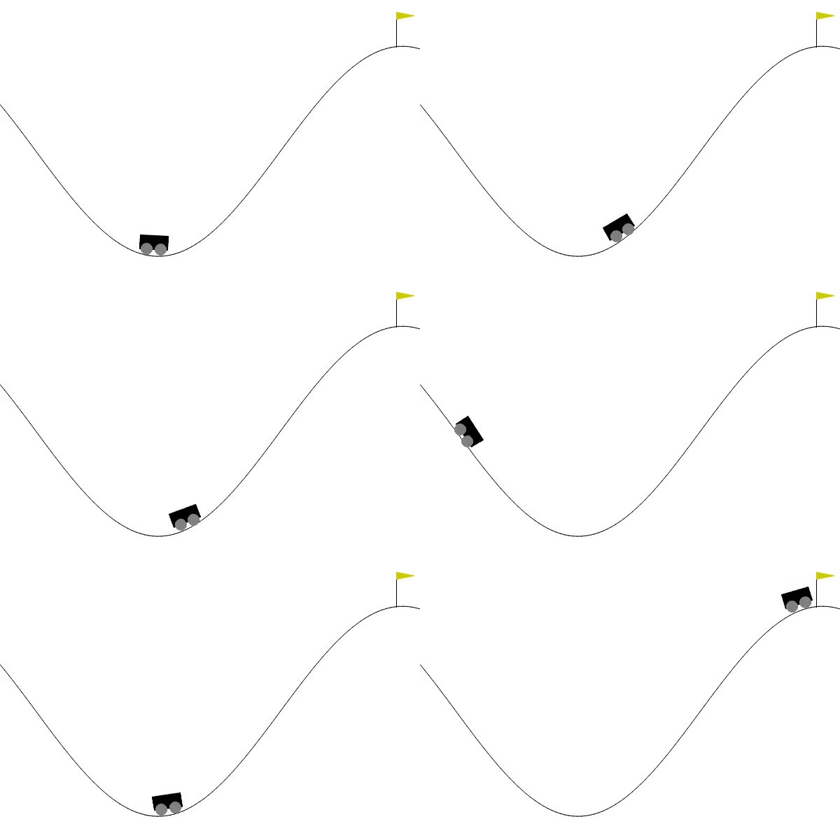 Now it's your turn to take the reins and improve the model. Dive into the code and make it your own. Tweak the hyperparameters, experiment with different model architectures, and see just how far you can push its performance. With a bit of creativity and persistence, you'll have that shuttle landing smoothly in no time!
5: Conclusion
In this article, we've explored the intricacies of Policy Gradient Methods in reinforcement learning, a powerful approach for training agents to make optimal decisions through direct optimization of policies. By delving into the theoretical foundations and practical implementations, we've laid out a comprehensive guide to understanding and applying these methods.
Reinforcement learning, especially through policy gradient methods, opens up vast possibilities for creating intelligent agents capable of learning from their interactions with the environment. As you continue to experiment and refine your models, remember that the key to success often lies in the details - careful design of networks, thoughtful reward shaping, and meticulous hyperparameter tuning.
References
- Towards Data Science (2024). The Math Behind Neural Network. https://medium.com/towards-data-science/the-math-behind-neural-networks-a34a51b93873
- Towards Data Science (2024). The Math Behind Recurrent Neural Networks. https://medium.com/towards-data-science/the-math-behind-recurrent-neural-networks-2de4e0098ab8
- Towards Data Science (2024). The Math Behind Convolutional Neural Network. https://medium.com/towards-data-science/the-math-behind-convolutional-neural-networks-6aed775df076
- Towards Data Science (2024). The Math Behind LSTM https://medium.com/towards-data-science/the-math-behind-lstm-9069b835289d
- Williams, R. J. (1992). Simple statistical gradient-following algorithms for connectionist reinforcement learning. Machine Learning, 8(3–4), 229–256.
- Silver, D., Lever, G., Heess, N., Degris, T., Wierstra, D., & Riedmiller, M. (2014). Deterministic policy gradient algorithms. In International Conference on Machine Learning (pp. 387–395). PMLR.
- Brockman, G., Cheung, V., Pettersson, L., Schneider, J., Schulman, J., Tang, J., & Zaremba, W. (2016). OpenAI Gym. arXiv preprint arXiv:1606.01540.
Register Now to Continue Reading
Unlock Towards Data Science with a Free Account
All articles on Towards Data Science are available to registered users. Create a free account today to access this article and thousands more.
Register for freeSign in to your account
 Written By
See all from Cristian Leo
Deep DivesDeep LearningMachine LearningPythonReinforcement Learning
Share This Article
Towards Data Science is a community publication. Submit your insights to reach our global audience and earn through the TDS Author Payment Program.
Write for TDS
Related Articles
Machine Learning
Bring Your ML Workloads To Production
Ram Vegiraju
December 31, 20215 min read
ChatGPT
How the humble prediction method shows us the way to Generative AI
Devesh Rajadhyax
April 25, 20239 min read
Deep Learning
From data gathering and preparation to model training and evaluation - Source code included.
Dario Radečić
October 5, 20219 min read
Machine Learning
Demystifying this often misunderstood theorem.
Amol Mavuduru
November 12, 20206 min read
Data Visualization
Is the ubiquitous original still the master?
Michael Clayton
January 20, 202418 min read
Deep Learning
As you know CNNs can be scaled if we require high computational power, but the larger the network more resources are required to train it...
Bharatdhyani
January 28, 20216 min read
Programming
Get rid of annoying SettingWithCopyWarning messages
Patrick Hoefler
December 21, 20228 min read
Machine Learning
You only define your destiny
Pranjal Saxena
October 19, 202010 min read
Machine Learning
In this article we will focus on a complete walk through of Python set operations.
Misha Sv
December 10, 20215 min read
Your home for data science and AI. The world's leading publication for data science, data analytics, data engineering, machine learning, and artificial intelligence professionals.
Subscribe to Our NewsletterWrite For TDS•About•Advertise•Privacy Policy•Terms of Use
© Insight Media Group, LLC 2026•The New Stack•roadmap.sh•Creator Network
Recommended Articles
Close