Logistic Regression: The Workhorse of Yes or No Problems

Remember the Swiggy late-order problem from a couple posts ago? Ten orders, distance in kilometers, and one simple label: was it late, yes or no. We tried fitting our usual straight line to it, and it fell apart: predictions wandered below 0 and above 1, and the line wasn't really giving us meaningful probabilities at all.

Last post, we met the fix for half of that problem. The sigmoid function, a curve that takes any number at all and always hands back something between 0 and 1. But we left it sitting there on its own, squashing random numbers like 2.73 into 0.939. It didn't know anything about distance, or orders, or lateness. It was just a shape.

Today we connect the two. We take the weighted sum we've used since the very first post, w times x plus b, and we feed it straight into the sigmoid. That combination has a name, and it is one of the most important models for yes-or-no prediction you'll come across.

The Idea in One Line

Here's the whole model, in a single formula.

P(y=1|x) = sigmoid(w × x + b)

Read that left side slowly, because the notation matters. P(y=1|x) means "the probability that y equals 1, given this particular x." In our case, y is whether an order is late, so y=1 means late and y=0 means not late. x is the distance. So the whole formula is really just asking, given how far away this order is, what's the probability it's late?

Notice what's inside the sigmoid. It's not some brand new formula. It's w times x plus b, the exact same weighted sum we've been computing since the first post in this series. Distance goes in, gets multiplied by a weight, has a bias added, and that raw number becomes z. Logistic regression uses that same weighted sum we already know from linear regression, but instead of using it directly as the answer, it passes it through the sigmoid, and out comes an estimated probability.

Seeing It Work, Before We Learn to Train It

Here's something worth being upfront about. We haven't yet learned how a machine finds the right w and b for a problem shaped like this one. The squared-error cost function we've used since post three doesn't actually work well here, and fixing that is a story for a future post.

But we can still see the model in action, using a w and b I've picked by hand, values that happen to fit our late-order data nicely. Let's use w = 2 and b = -11, and see what happens.

Distance	z = 2x − 11	P(late) = sigmoid(z)	Actually Late?
1 km	−9	0.0001	No
2 km	−7	0.0009	No
3 km	−5	0.0067	No
4 km	−3	0.0474	No
5 km	−1	0.2689	No
6 km	+1	0.7311	Yes
7 km	+3	0.9526	Yes
8 km	+5	0.9933	Yes
9 km	+7	0.9991	Yes
10 km	+9	0.9999	Yes

Unlike our straight-line model, every output here stays between 0 and 1. This dataset is deliberately clean, so the transition from "no" to "yes" looks almost perfect. Real delivery data will be messier.

Checking One Value By Hand

Let's actually work through the 6 km row ourselves, the same way we've checked every formula in this series.

z = w × x + b
z = 2 × 6 + (-11)
z = 12 - 11
z = 1

Now we pass that z into the sigmoid formula from last post.

P(late) = 1 / (1 + e^-1)

e to the power of -1 is roughly 0.3679, so:

P(late) = 1 / (1 + 0.3679)
P(late) = 1 / 1.3679
P(late) = 0.7311

A 73.1% chance of being late, for an order 6 kilometers away. That matches the table exactly, and it's a number you could actually say out loud to someone and have it make sense.

Turning This Into Code

The whole model is barely more code than the sigmoid function was on its own.

import numpy as np

def sigmoid(z):
    return 1 / (1 + np.exp(-z))


def logistic_regression_predict(x, w, b):
    z = w * x + b
    return sigmoid(z)


distances = np.array([1, 2, 3, 4, 5, 6, 7, 8, 9, 10], dtype=float)
late = np.array([0, 0, 0, 0, 0, 1, 1, 1, 1, 1], dtype=float)

w, b = 2, -11
probabilities = logistic_regression_predict(distances, w, b)

for d, p, actual in zip(distances, probabilities, late):
    print(f"{d:.0f} km -> P(late) = {p:.4f}  (actually {'late' if actual else 'not late'})")

Running this prints the exact same numbers from our table above. The function itself is just two lines: compute z the familiar way, then squash it with sigmoid. The sigmoid curve and the weighted sum were both built in earlier posts. Logistic regression is really just those two ideas, standing on each other's shoulders.

One Thing Worth Noticing Before We Move On

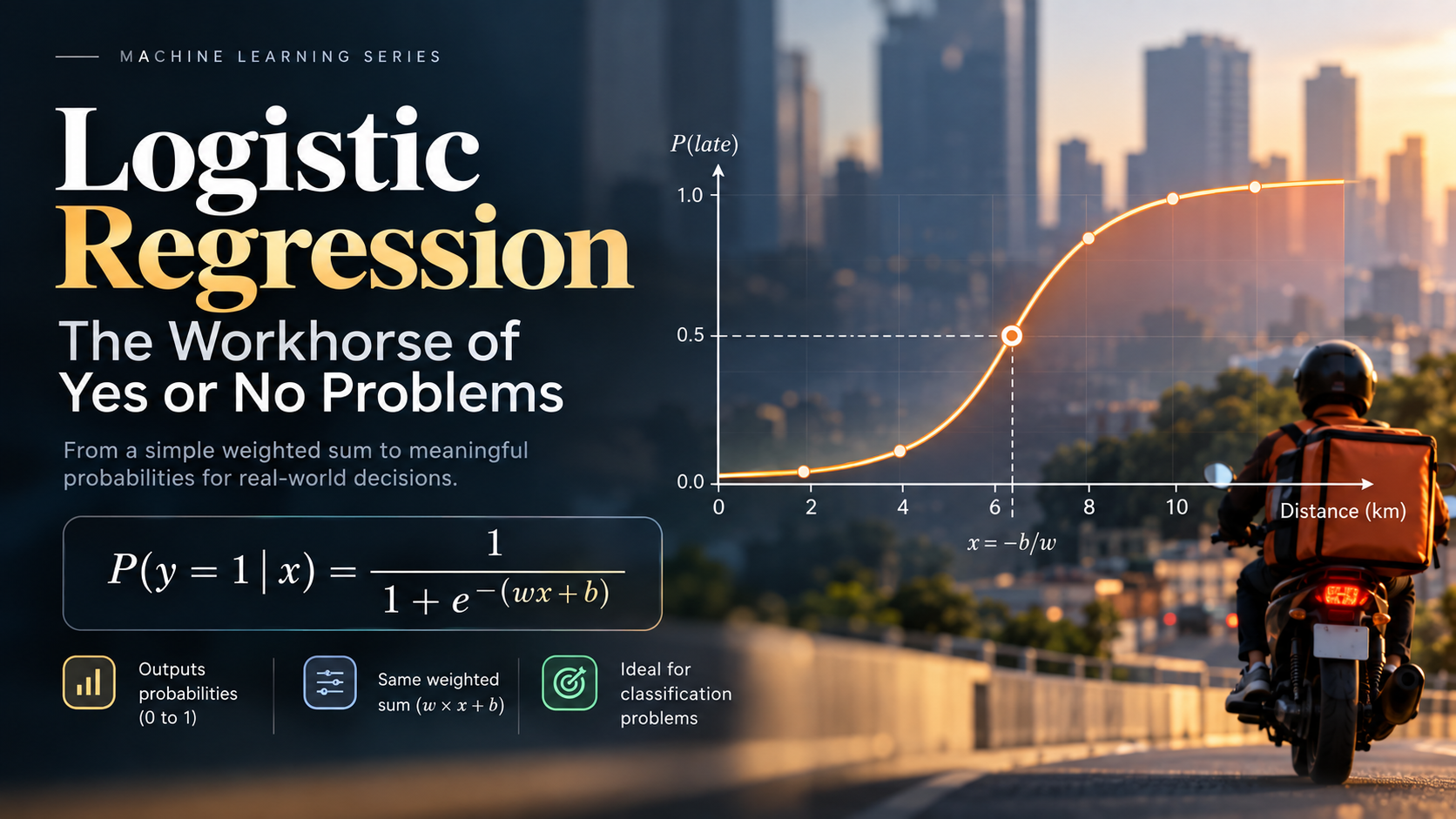
The model gives us a probability, not a decision. If we use 0.5 as our classification threshold, probabilities below 0.5 become "no" and probabilities above 0.5 become "yes." Whenever the model's z reaches 0, the sigmoid outputs exactly 0.5. For our one-feature model, that happens where w × x + b = 0, which we can rearrange to:

x = -b / w

For our numbers, that's x = -(-11) / 2 = 5.5 km, right in the middle of where our table flips from "no" to "yes."

The magnitude of w controls how sharply the probability changes as x changes, a larger |w| makes the curve steeper, while b shifts where that steep part sits along the x-axis. (A negative w would flip the direction entirely, but that's a story for another day.)

If we use 0.5 as our classification threshold, at what point does the model stop saying "probably no" and start saying "probably yes"? That's the piece we'll isolate in the next post.

Where We Go From Here

We've handed you working weights twice in a row now, first the linear regression posts, and now this one. That's fair to be a little suspicious of. Before we finally learn how a machine finds these weights on its own, there's one more idea worth seeing clearly, the exact line where the model's decision flips from one answer to the other. Next time, we'll draw that line ourselves, using a completely different problem: a food delivery app deciding, in real time, whether to switch on surge pricing.

The full notebook for this post, including every calculation above, is up on GitHub here: github.com/tharun-pandya/Machine-Learning-Blog-Series/blob/main/Logistic_Regression.ipynb

See you in the next one.