A few months ago, I locked myself out of my own apartment.
I stood outside, called a locksmith, and watched him work. He looked at the lock, cut a fresh key, turned it, and — click — the door opened. One clean, precise action, completely undone.
Here's a question worth actually sitting with: why did that work? Why could he undo the lock, but if that same lock had been crushed, melted, or welded shut, no locksmith on the planet could bring it back to "unlocked" again?
The answer is simple once you say it out loud: a normal turning lock is a reversible action. Twist one way, it locks. Twist the exact opposite way, it unlocks. But crushing a lock isn't reversible — no matter how skilled the locksmith is, there's no "opposite" action that un-crushes metal back into a working lock. Some actions can be undone. Some actions destroy information so completely that undoing them is simply impossible, no matter how clever you are.
This single idea — some actions can be undone, some can't, and you can actually tell in advance which is which — is the entire subject of this blog. And it turns out, this exact idea sits at the very heart of how Machine Learning models "learn," how camera apps fix a distorted photo, and even hints at something surprisingly true about your own memory.
In the earlier blogs of this series, we learned to add, subtract, mask, and multiply matrices. Today, we go one level deeper and ask: when you multiply your data by a matrix, what is actually happening to it? Is it just numbers shuffling around, or is something bigger going on — something geometric, something you could almost picture with your eyes closed?
By the end of this blog, you will understand:
What a linear transformation genuinely is — what multiplying by a matrix actually does to your data, in a way you can picture
What the determinant tells you, before you even attempt anything else, about whether a transformation is reversible
What the matrix inverse is, how to build it from scratch, and why it's the mathematical version of the locksmith's key
Real, low-level examples from camera lens correction, face recognition, and how your own memory works
Why this trio, quietly, is the mathematical backbone of linear regression, PCA, and how neural networks reshape raw data into decisions
Let's take this slowly, one idea at a time.
Picture a flat rubber sheet with a perfectly even grid drawn on it — neat little squares, all the same size, evenly spaced, like graph paper.
Now imagine grabbing that sheet with both hands and doing something to it — stretching it wider, spinning it slightly, or squashing it thinner. Watch what happens to the grid lines. They might get longer or shorter. The squares might turn into rectangles, or lean into diamonds. But — and this is the important part — the lines stay perfectly straight, and they stay evenly spaced relative to each other. No line bends into a curve. No two originally-parallel lines suddenly cross each other.
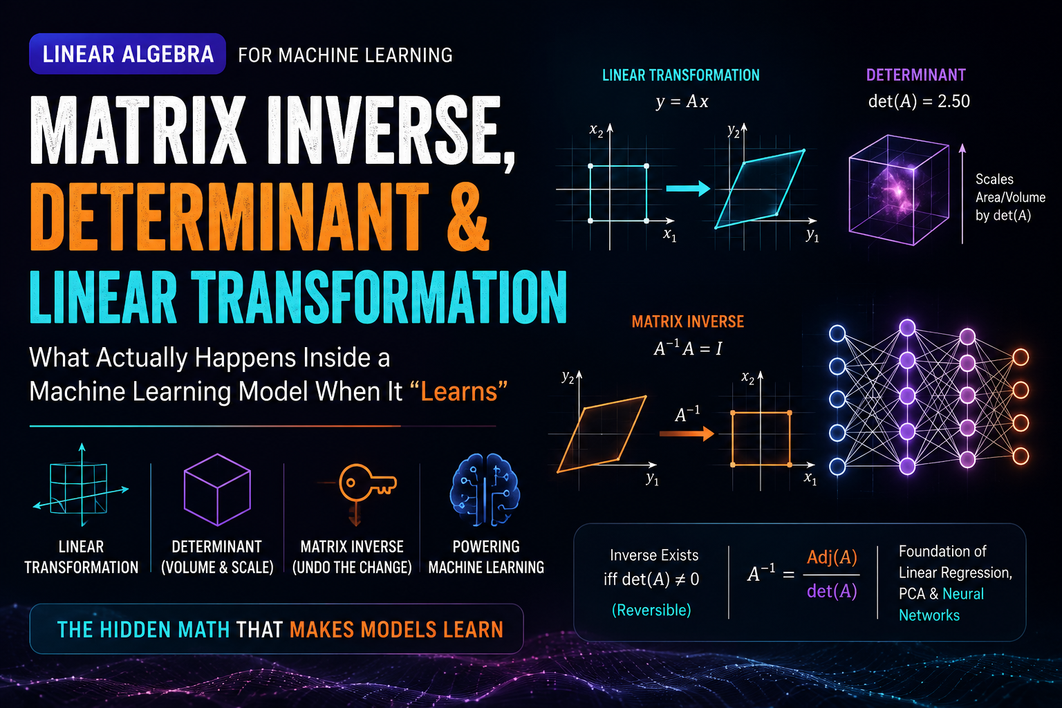
That specific kind of movement — stretching, rotating, or squashing, while keeping straight lines straight and spacing even — is called a linear transformation. And here's the sentence that ties this entire blog series together, so read it twice:
Every time you multiply a vector (or a whole matrix of data) by another matrix, using real matrix multiplication, you are applying a linear transformation to it. The matrix itself is nothing but a stored instruction — "stretch this way, rotate that much, squash this direction" — waiting to be applied to whatever numbers you feed it.
Let's use a small, concrete matrix as our "instruction," and a single vector as the thing being transformed.
import numpy as np

A = np.array([[12, 3, 13, 6],
              [1, 15, 7, 5],
              [4, 11, 4, 8],
              [18, 2, 6, 8]])

x = np.array([[1], [2], [3], [4]])

def transformation(a, x):
    result = np.zeros((a.shape[0], x.shape[1]))
    for i in range(x.shape[0]):
        for j in range(a.shape[0]):
            result[i] += a[i, j] * x[j]
    return result

print(transformation(A, x))
[[81.]
 [72.]
 [70.]
 [72.]]
Look closely at what this code is actually doing — it's the exact matrix multiplication you learned in the last blog, just applied to a single column of numbers (a vector) instead of a full grid. Our starting vector was [1, 2, 3, 4]. After being multiplied by matrix A, it "moved" to a brand new position: [81, 72, 70, 72].
Nothing about this feels dramatic when you just look at the numbers. But picture it the rubber-sheet way instead: imagine [1, 2, 3, 4] as a single point sitting somewhere on that grid. Multiplying it by A is exactly like grabbing the whole sheet and stretching, rotating, or squashing it according to the "instructions" written inside A — and that point on the sheet gets carried along to a brand new location, [81, 72, 70, 72], purely because the sheet itself moved underneath it.
1. Rotating and resizing a photo (Computer Vision)
When you rotate a photo 15 degrees in an editing app, or resize it to fit an Instagram story, the app isn't magically "redrawing" the image. It takes the (x, y) coordinate of every single pixel — imagine each pixel's position as a tiny 2-number vector — and multiplies it by a small rotation-and-scaling matrix. Every pixel gets carried to a new position, exactly like the point on our rubber sheet, and the collection of all these moved pixels is your rotated, resized photo. Do this for a few million pixels, and it happens instantly, every time you pinch-zoom or rotate a photo on your phone.
2. Face filters stretching your face into a cartoon (Computer Vision)
Those "big eyes, small chin" cartoon-style filters on Snapchat and Instagram work by taking the coordinates of your detected face mesh (remember the triangle mesh from the last blog) and applying a carefully designed linear transformation matrix that stretches certain regions (the eyes) and shrinks others (the chin), while keeping the overall structure of the face recognizably intact. It's the exact same rubber-sheet stretching idea, just applied specifically and cleverly to different regions of your face.
3. Every single layer of a neural network reshaping data (Deep Learning, Translation Apps)
Here's the big one, worth sitting with. When a translation app processes your sentence, or a face recognition system processes your photo, the raw input data (word numbers, or pixel numbers) doesn't stay in its original form the whole way through. It passes through many layers, one after another, and each layer applies its own linear transformation — its own "stretch, rotate, squash" instruction, learned automatically during training (a topic for a future blog, don't worry about the word "training" itself right now) — gradually reshaping the raw data into a new form where the final answer (which word comes next, whose face this is) becomes far easier to read off directly.
This is genuinely one of the most useful mental pictures you can carry forward from this entire series:
A neural network is really just a long chain of linear transformations, each one reshaping the data a little more, until the final shape makes the answer obvious.
It's rubber sheets, stacked on top of rubber sheets, each one stretched slightly differently, until what started as a meaningless grid of pixel brightness numbers ends up perfectly shaped to reveal "this is a photo of a cat" or "this sentence is happy, not sad."
But here's a question this immediately raises, and it's the reason the rest of this blog exists: if a transformation reshapes your data, can you always get the original data back? Sometimes yes. Sometimes, shockingly, no. Let's find out how to tell the difference, before we ever attempt to undo anything.
Go back to the rubber sheet. If you stretch it gently — say, pulling it a little wider — every original square grows a bit bigger, but you can still clearly make out every original square's shape. Crucially, if you knew exactly how much you stretched it, you could pull it back the opposite way and get the exact original grid back, perfectly.
But now imagine squashing the sheet so hard, from one direction, that it completely flattens into a single straight line — or worse, into a single point. Now, many, many different original squares have all been crushed down onto that same flat line, or that same single point. If someone showed you only that flattened result and asked, "which original square was this?" — you genuinely could not answer. Multiple different starting points have been merged into one, indistinguishable, final position. There's no way back. The information about which square it originally was is gone, permanently.
The determinant is a single number, calculated directly from a matrix, that tells you — before you ever attempt anything — which of these two situations you're facing.
If a matrix's determinant is exactly zero, the transformation it represents crushes information down so completely that undoing it is mathematically impossible. If the determinant is any number other than zero, the transformation is fully reversible.
Here's a genuinely useful, low-level example. Imagine a self-driving car with two nearly-identical distance sensors, both facing forward, mounted just a few centimeters apart. If both sensors, for some reason, always report exactly the same distance reading in every situation (say, due to a wiring mistake accidentally connecting them to the same signal), then the "matrix" describing these two sensor readings together has effectively collapsed into just one piece of real information, duplicated twice. Mathematically, this shows up as a determinant of zero — a strong, precise, mathematical warning sign that says, "you think you have two independent pieces of information here, but you actually only have one, and part of what you thought you knew is unrecoverable, because it was never really separate to begin with."
This exact warning sign — a zero, or very close to zero, determinant — is one of the very first things engineers check for when building systems that rely on combining multiple sensors or multiple features, precisely because it flags hidden, wasted redundancy before it causes a bigger, more confusing failure downstream.
For a small, 2-by-2 matrix, the determinant has a direct, simple formula:
For a 2x2 matrix   [a  b]
                    [c  d]

determinant = (a × d) − (b × c)
Let's fully work through a real example by hand.
Matrix =   [2   1]
           [1   3]
determinant = (2 × 3) − (1 × 1)
            = 6 − 1
            = 5
Since 5 is not zero, this transformation is fully reversible — nothing gets permanently crushed. Good news; we'll actually undo this exact matrix ourselves in Part 3.
Now let's see what a zero determinant genuinely looks like, using an example built from real, whole numbers, so you can verify it yourself:
Matrix =    [1   2   3]
            [4   5   6]
            [7   8   9]
If you look closely at this matrix, you'll notice something quietly suspicious: each row is simply the row above it, plus 3, added to every number (1,2,3 then 4,5,6 then 7,8,9). The third row isn't really "new" information — it's secretly just a combination of the first two rows. This hidden redundancy is exactly the kind of thing a zero determinant is built to catch. And indeed, if you calculate it (we'll show the code shortly), this matrix's determinant comes out to exactly zero.
For matrices bigger than 2-by-2, the determinant is calculated by breaking the matrix down into smaller and smaller pieces — a process called cofactor expansion — repeatedly, until you're only left with tiny 2x2 or 1x1 pieces you already know how to solve directly. You genuinely never need to memorize this process by hand for anything beyond a small textbook example — but let's still build it from scratch in code, so you can see, honestly, that there's no hidden magic inside np.linalg.det().
import numpy as np

def det(a):
    if len(a) == 1:
        return a[0][0]
    if len(a) == 2:
        return a[0][0] * a[1][1] - a[0][1] * a[1][0]

    result = 0
    for col in range(len(a)):
        minor = [
            [a[row][c] for c in range(len(a)) if c != col]
            for row in range(1, len(a))
        ]
        result += ((-1) ** col) * a[0][col] * det(np.array(minor))

    return result
Let's unpack this slowly, piece by piece, because at first glance this looks intimidating and it really isn't.
if len(a) == 1 and if len(a) == 2 — these are our two simple "base cases," the ones we can solve directly using the small formula above, without needing to break the matrix down any further.
For anything bigger than 2x2, the function looks at the first row, one number at a time (a[0][col]), and for each of those numbers, it builds a smaller matrix called minor — this is simply the original matrix with that number's entire row and column removed.
It then calls det() on that smaller minor matrix — this is the function calling itself, on a smaller piece of the problem, a technique called recursion. Think of it like those Russian nesting dolls — each doll opens to reveal a smaller doll of the exact same shape, until you reach the smallest one that can't be opened any further (our 1x1 and 2x2 base cases).
The ((-1) ** col) part just means the sign flips back and forth (positive, negative, positive, negative...) as we move across the row — this is a specific mathematical detail of how cofactor expansion is defined, and while it's worth knowing it exists, you don't need to memorize exactly why it alternates to use this code correctly.
Let's test it against NumPy's own built-in version, to make sure it genuinely works:
A = np.array([[12, 3, 13, 6],
              [1, 15, 7, 5],
              [4, 11, 4, 8],
              [18, 2, 6, 8]])

print("hand-built:", det(A), "\t numpy:", np.linalg.det(A))
# hand-built: 6706    numpy: 6705.999999999999
That tiny difference (6706 versus 6705.999...) is nothing to worry about — it's just a normal, expected side-effect of how computers store decimal numbers with a small amount of built-in imprecision, called floating-point rounding. Both answers genuinely mean the same thing.
Now let's test our earlier redundant matrix, the one with rows that secretly repeat information:
B = np.array([[1, 2, 3],
              [4, 5, 6],
              [7, 8, 9]])

print("hand-built:", det(B), "\t numpy:", np.linalg.det(B))
# hand-built: 0    numpy: -9.5e-16  (essentially zero)
Exactly as we predicted just by eyeballing the pattern in the rows — the determinant comes out to zero (NumPy's tiny -9.5e-16 is so close to zero it's effectively zero, again just floating-point rounding noise). This matrix genuinely, mathematically destroys information the moment you use it in a transformation, and there is no possible "undo" matrix that could bring back what's lost.
1. Checking if a face recognition model's "faceprints" are actually useful (Computer Vision)
Remember the 128-number face embeddings from the last blog? Imagine, hypothetically, a badly designed face recognition system where several of those 128 numbers always ended up being near-identical copies of each other, no matter whose face it was looking at — essentially wasted, redundant information, contributing nothing new. Engineers can use determinant-based checks (on the relationships between these numbers, across many faces) to catch this kind of hidden redundancy early, before it quietly causes the system to struggle telling two different people apart.
2. Detecting redundant, near-duplicate sensor data (Self-driving cars, Robotics)
Exactly as in our earlier example — if two sensors are secretly reporting the same information in different disguises, the mathematics built on top of their combined readings develops a near-zero determinant, acting as an early, automatic warning sign of wasted, duplicated data.
3. Deciding if a distorted photo can even theoretically be corrected (Computer Vision, camera apps)
If a photo has been so severely distorted or compressed that entire regions of visually different content have been crushed down into identical, indistinguishable blocks of pixels, no "undo" algorithm, however clever, can perfectly restore the original detail. This is directly connected to the idea of a zero determinant — once information is truly, completely crushed together, no mathematical trick can separate it back out. This is precisely why, when you excessively zoom into a low-quality photo, you get blurry, blocky mush instead of your original sharp detail returning — the information genuinely, permanently, isn't there to recover anymore.
Once you know, using the determinant, that a transformation can be undone, the matrix inverse is the actual, precise key that undoes it — exactly like the locksmith's freshly cut key from the very start of this blog.
Multiplying a matrix by its own inverse gives you the identity matrix — a special matrix (all
1s along the diagonal,0s everywhere else) that represents "doing absolutely nothing" — the exact mathematical equivalent of multiplying an ordinary number by 1.
This matters enormously in practice because a huge number of real problems boil down to exactly this shape: "I know the result of a transformation. I know what transformation was applied. Now, what was the original data before the transformation happened?" Whenever a problem takes this shape — written as A @ x = b, meaning "some matrix A, multiplied by an unknown x, gives a known result b" — the inverse gives you a direct, precise way to solve for that unknown x:
x = A⁻¹ @ b
The inverse is built from two ingredients you've already met: the determinant, and something called the adjugate — a slightly more elaborate cousin of the determinant, built using the exact same "cofactor" idea, just organized a little differently.
import numpy as np

def det(A):
    rows, cols = A.shape
    if rows == 1:
        return A[0][0]
    if rows == 2:
        return A[0][0]*A[1][1] - A[0][1]*A[1][0]
    result = 0
    for i in range(rows):
        mat = np.zeros((rows-1, cols-1))
        n = 0
        for j in range(1, rows):
            m = 0
            for k in range(cols):
                if k == i:
                    continue
                mat[n][m] = A[j][k]
                m += 1
            n += 1
        result += ((-1)**i) * A[0][i] * det(mat)
    return result

def adjugate(matrix):
    if len(matrix) == 2:
        res = np.zeros((2, 2))
        res[0, 0] = matrix[1, 1]
        res[0, 1] = -matrix[0, 1]
        res[1, 0] = -matrix[1, 0]
        res[1, 1] = matrix[0, 0]
        return res
    # for matrices larger than 2x2, the same cofactor idea extends further —
    # we're keeping this example to a 2x2 case to stay clear and readable

def inverse(A):
    det_A = det(A)
    return (1 / det_A) * adjugate(A)
Look closely at that final function, inverse(A). It's genuinely doing something you could describe in one plain-English sentence: "take the adjugate, and shrink or grow it according to 1 divided by the determinant." This single detail is also exactly why a zero determinant makes an inverse completely impossible to compute — dividing by zero is undefined, mathematically forbidden, and Python (like any calculator) will refuse to do it, giving you an error instead of a nonsensical answer. This is the deep, precise reason a zero-determinant matrix truly cannot be undone — not just "practically difficult," but genuinely, mathematically impossible.
Remember our simple, fully-reversible matrix from Part 2?
Matrix =   [2   1]
           [1   3]      (determinant was 5, safely non-zero)
a = np.array([[2, 1], [1, 3]])

a_inverse = inverse(a)
print(a_inverse)
[[ 0.6 -0.2]
 [-0.2  0.4]]
Now, the real test — does multiplying the original matrix by this inverse genuinely give us back the "do nothing" identity matrix?
print(np.dot(a, a_inverse).astype(int))
[[1 0]
 [0 1]]
Exactly the identity matrix, precisely as we hoped. The original transformation, and its inverse, cancel each other out perfectly — genuinely no different, mathematically, from turning a key one way to lock a door, and turning it the exact opposite way to unlock it again.
In real, professional Machine Learning work, you'll essentially never hand-build an inverse this way for anything beyond a small teaching example — NumPy's np.linalg.inv(A) handles it far more efficiently and reliably for large, real-world matrices. But now, genuinely, you know exactly what's happening the moment you type that one line of code.
1. Predicting house prices — solving for the "best formula" directly (Machine Learning, tying back to blog 3)
Remember our house price example from earlier in this series — bedrooms, bathrooms, and square footage predicting price? Finding the single "best" formula that fits a whole dataset of past house sales (this exact process is called linear regression, and don't worry, we'll dedicate an entire future blog to properly unpacking how a model "learns" this formula) has a direct, one-step mathematical solution, and matrix inverse sits right at its center:
best_formula_weights = inverse(Xᵀ @ X) @ Xᵀ @ actual_prices
You don't need to memorize this formula right now — just notice that the word "inverse" appears directly inside it. Solving for the single best price-prediction formula, across potentially thousands of past house sales at once, genuinely depends on being able to compute a matrix inverse.
2. Correcting fisheye and lens distortion in phone cameras (Computer Vision)
Wide-angle and "fisheye" camera lenses (common in phone ultra-wide cameras, action cameras, and security cameras) bend straight lines into curves, purely because of how the physical lens glass is shaped. Camera software knows, in advance, exactly what distortion transformation that specific lens applies — this is measured carefully during the camera's design and calibration. To give you a normal-looking, straight-lined photo, the software applies the inverse of that known distortion transformation, mathematically "unbending" the image back to how it would have looked through an ordinary, undistorted lens. Every time your phone gives you a straight-edged, undistorted ultra-wide photo, an inverse transformation almost certainly just ran, silently, correcting for the lens's natural bending.
3. Figuring out a robot's exact position from multiple distance readings (Robotics)
When a robot (or a self-driving car) needs to figure out its exact position using several distance measurements from known landmarks (a process related to GPS and a technique sometimes called triangulation), the underlying math frequently reduces to solving exactly the A @ x = b shape mentioned earlier — where x is the robot's unknown position, and matrix inverse (or a more numerically careful equivalent used in real systems) is precisely the tool used to solve for it directly.
One honest, important caution worth carrying forward: computing a matrix inverse directly can become slow and less numerically reliable for very large matrices. Real-world ML libraries very often use smarter, more efficient techniques that achieve the same goal — solving for the unknown — without literally computing a full inverse matrix by hand. But the core idea, "the inverse is the precise mathematical key that undoes a transformation," remains exactly the right mental model for understanding what those more efficient techniques are actually approximating underneath.
Take a moment here, because you've genuinely covered a lot of ground across these six blogs. Let's see it all laid out in one place.
You learned why Machine Learning needs linear algebra at all — because computers only understand numbers, and linear algebra is the language for organizing and manipulating large groups of numbers efficiently.
You learned what a vector is — one single example, described entirely as a list of numbers.
You learned what a matrix is — many vectors, stacked together into one organized table.
You learned addition, subtraction, and element-wise multiplication — the simple, "position matches position" operations that combine, compare, and mask data.
You learned matrix multiplication, transpose, and cross product — the operations that genuinely weigh, combine, and reorient data into something new.
And now, you understand linear transformation, determinant, and matrix inverse — what a matrix truly does to your data geometrically, whether that action can be undone, and exactly how to undo it if it can.
| Concept | What it tells you, in one line |
|---|---|
| Linear transformation | What multiplying by a matrix actually does to your data — stretch, rotate, or squash it |
| Determinant | Whether that action can be undone at all, or whether information has been destroyed forever |
| Matrix inverse | The exact, precise action that undoes it, whenever undoing is genuinely possible |
Put together, honestly, this is real, working mathematical understanding of what's happening inside linear regression, inside PCA, and inside the forward pass of a neural network — not "trust the library, it just works," but a genuine, ground-level understanding of the actual arithmetic quietly running underneath.
Here's something worth closing on, because I think it's the most quietly profound idea in this entire blog.
Think about your own memory for a moment. When you remember a childhood birthday party, you don't actually replay a perfect, complete recording of that day. Your brain stores a compressed, simplified version — a handful of key details (a cake, a certain song, a particular feeling) — and every other tiny detail (the exact angle of the sunlight, the precise words your cousin said, what you were wearing on your left foot) is, quite simply, gone. Permanently. Crushed away, the same way our redundant, zero-determinant matrix crushed different starting squares down into one indistinguishable, unrecoverable position.
Your brain, in other words, applies something remarkably like a non-reversible transformation to your own experiences, every single day, without asking your permission — keeping what it judges important, and letting the rest collapse away forever, with no "inverse" available to bring back what's lost. This isn't a flaw in your memory. It's almost certainly a deliberate, efficient design, honed by millions of years of evolution — full, perfect recall of every waking second would be an unimaginable, overwhelming amount of information to carry around.
Machine Learning models, in a strange and genuinely fascinating way, do something remarkably similar on purpose. A face recognition system doesn't need to remember every single pixel of your face perfectly — it deliberately compresses your face down into just 128 carefully-chosen numbers, discarding almost everything else, because those 128 numbers happen to be exactly enough to tell you apart from millions of other people. That deliberate act of throwing away the unimportant and keeping only what matters — the same core idea as a determinant collapsing information, done on purpose, carefully, usefully — is arguably the single biggest reason modern Machine Learning models work at all. Understanding this math, genuinely, isn't just a technical skill. It's a small window into how information itself — in a phone, in an algorithm, and quite possibly inside your own head — decides, silently, every single day, what's worth keeping and what's allowed to disappear.
We started this entire series by asking one simple question: why does Machine Learning even need linear algebra? Six blogs later, you now have a genuine, working answer — because every Machine Learning model, from the simplest house-price predictor to the largest translation and chat AI systems in the world, is fundamentally built from exactly the operations covered across this series, applied over and over, at a truly enormous scale, reshaping raw numbers into useful, real-world answers.
The natural next stop from here is eigenvalues and eigenvectors — a genuinely fascinating idea that says: every transformation has certain special directions it never rotates or bends, only stretches or shrinks along. This single idea is precisely what powers PCA (a technique for simplifying huge, complicated datasets down to their most important patterns), what makes certain kinds of image compression possible, and — genuinely fascinating — what powered an early, famous version of one of the most successful face recognition techniques ever built, sometimes nicknamed "Eigenfaces," where a person's face is described not by 128 abstract numbers, but by exactly these special stretching directions.
If matrices, throughout this series, have been the "actions" — the stretching, squashing, and combining — eigenvectors are about to show you the one direction each of those actions can never bend, only stretch. That's a strange, beautiful enough idea to deserve its very own blog.
See you there.