保留正文与补采附件。源页面当前未重新核验;具体限制见交付清单。
 We value your privacy
We use cookies to enhance your browsing experience, serve personalised ads or content, and analyse our traffic. By clicking "Accept All", you consent to our use of cookies.
Customise Reject All Accept All
Customise Consent Preferences
 We use cookies to help you navigate efficiently and perform certain functions. You will find detailed information about all cookies under each consent category below.
The cookies that are categorised as "Necessary" are stored on your browser as they are essential for enabling the basic functionalities of the site. ... Show more
NecessaryAlways Active
Necessary cookies are required to enable the basic features of this site, such as providing secure log-in or adjusting your consent preferences. These cookies do not store any personally identifiable data.
-
Cookie
BCTempID
-
Duration
10 minutes
-
Description
No description available.
-
Cookie
__cf_bm
-
Duration
1 hour
-
Description
This cookie, set by Cloudflare, is used to support Cloudflare Bot Management.
-
Cookie
AWSALBCORS
-
Duration
7 days
-
Description
Amazon Web Services set this cookie for load balancing.
-
Cookie
_cfuvid
-
Duration
session
-
Description
Cloudflare sets this cookie to track users across sessions to optimize user experience by maintaining session consistency and providing personalized services
-
Cookie
li_gc
-
Duration
6 months
-
Description
Linkedin set this cookie for storing visitor's consent regarding using cookies for non-essential purposes.
-
Cookie
__hssrc
-
Duration
session
-
Description
This cookie is set by Hubspot whenever it changes the session cookie. The __hssrc cookie set to 1 indicates that the user has restarted the browser, and if the cookie does not exist, it is assumed to be a new session.
-
Cookie
__hssc
-
Duration
1 hour
-
Description
HubSpot sets this cookie to keep track of sessions and to determine if HubSpot should increment the session number and timestamps in the __hstc cookie.
-
Cookie
wpEmojiSettingsSupports
-
Duration
session
-
Description
WordPress sets this cookie when a user interacts with emojis on a WordPress site. It helps determine if the user's browser can display emojis properly.
-
Cookie
BCSessionID
-
Duration
1 year 1 month 4 days
-
Description
Blueconic sets this cookie as a unique identifier for the BlueConic profile.
-
Cookie
_octo
-
Duration
1 year
-
Description
No description available.
-
Cookie
logged_in
-
Duration
1 year
-
Description
No description available.
-
Cookie
__Secure-YEC
-
Duration
past
-
Description
YouTube sets this cookie to stores the user's video player preferences using embedded YouTube video
-
Cookie
__eoi
-
Duration
6 months
-
Description
Description is currently not available.
-
Cookie
AWSALBTGCORS
-
Duration
7 days
-
Description
No description available.
-
Cookie
login-status-p
-
Duration
past
-
Description
Description is currently not available.
-
Cookie
AWSALBTG
-
Duration
7 days
-
Description
No description available.
-
Cookie
csrf_token
-
Duration
session
-
Description
No description available.
-
Cookie
token_v2
-
Duration
1 day
-
Description
Description is currently not available.
-
Cookie
D
-
Duration
1 year
-
Description
Description is currently not available.
-
Cookie
PHPSESSID
-
Duration
session
-
Description
This cookie is native to PHP applications. The cookie stores and identifies a user's unique session ID to manage user sessions on the website. The cookie is a session cookie and will be deleted when all the browser windows are closed.
-
Cookie
VISITOR_PRIVACY_METADATA
-
Duration
6 months
-
Description
YouTube sets this cookie to store the user's cookie consent state for the current domain.
-
Cookie
cookietest
-
Duration
session
-
Description
The cookietest cookie is typically used to determine whether the user's browser accepts cookies, essential for website functionality and user experience.
-
Cookie
__Host-airtable-session
-
Duration
1 year
-
Description
This cookie is used to enable us to integrate the services of Airtable.
-
Cookie
__Host-airtable-session.sig
-
Duration
1 year
-
Description
This cookie is used to enable us to integrate the services of Airtable.
-
Cookie
m
-
Duration
1 year 1 month 4 days
-
Description
Stripe sets this cookie for fraud prevention purposes. It identifies the device used to access the website, allowing the website to be formatted accordingly.
-
Cookie
BIGipServer*
-
Duration
session
-
Description
Marketo sets this cookie to collect information about the user's online activity and build a profile about their interests to provide advertisements relevant to the user.
-
Cookie
__cfruid
-
Duration
session
-
Description
Cloudflare sets this cookie to identify trusted web traffic.
-
Cookie
_GRECAPTCHA
-
Duration
6 months
-
Description
Google Recaptcha service sets this cookie to identify bots to protect the website against malicious spam attacks.
-
Cookie
__Secure-YNID
-
Duration
6 months
-
Description
Google cookie used to protect user security and prevent fraud, especially during the login process.
-
Cookie
cookieyes-consent
-
Duration
1 year
-
Description
CookieYes sets this cookie to remember users' consent preferences so that their preferences are respected on subsequent visits to this site. It does not collect or store any personal information about the site visitors.
Functional
Functional cookies help perform certain functionalities like sharing the content of the website on social media platforms, collecting feedback, and other third-party features.
-
Cookie
lidc
-
Duration
1 day
-
Description
LinkedIn sets the lidc cookie to facilitate data center selection.
-
Cookie
brw
-
Duration
1 year
-
Description
No description available.
-
Cookie
brwConsent
-
Duration
5 minutes
-
Description
Description is currently not available.
-
Cookie
WMF-Uniq
-
Duration
1 year
-
Description
Description is currently not available.
-
Cookie
loom_anon_comment
-
Duration
1 year
-
Description
No description available.
-
Cookie
loom_referral_video
-
Duration
session
-
Description
Description is currently not available.
-
Cookie
VISITOR_INFO1_LIVE
-
Duration
6 months
-
Description
A cookie set by YouTube to measure bandwidth that determines whether the user gets the new or old player interface.
-
Cookie
yt-remote-connected-devices
-
Duration
Never Expires
-
Description
YouTube sets this cookie to store the user's video preferences using embedded YouTube videos.
-
Cookie
ytidb::LAST_RESULT_ENTRY_KEY
-
Duration
Never Expires
-
Description
The cookie ytidb::LAST_RESULT_ENTRY_KEY is used by YouTube to store the last search result entry that was clicked by the user. This information is used to improve the user experience by providing more relevant search results in the future.
-
Cookie
yt-remote-device-id
-
Duration
Never Expires
-
Description
YouTube sets this cookie to store the user's video preferences using embedded YouTube videos.
-
Cookie
yt-remote-session-name
-
Duration
session
-
Description
The yt-remote-session-name cookie is used by YouTube to store the user's video player preferences using embedded YouTube video.
-
Cookie
yt-remote-fast-check-period
-
Duration
session
-
Description
The yt-remote-fast-check-period cookie is used by YouTube to store the user's video player preferences for embedded YouTube videos.
-
Cookie
yt-remote-session-app
-
Duration
session
-
Description
The yt-remote-session-app cookie is used by YouTube to store user preferences and information about the interface of the embedded YouTube video player.
-
Cookie
yt-remote-cast-available
-
Duration
session
-
Description
The yt-remote-cast-available cookie is used to store the user's preferences regarding whether casting is available on their YouTube video player.
-
Cookie
yt-remote-cast-installed
-
Duration
session
-
Description
The yt-remote-cast-installed cookie is used to store the user's video player preferences using embedded YouTube video.
-
Cookie
cp_session
-
Duration
3 months
-
Description
Codepen sets this cookie for Help systems found in the website.
-
Cookie
loid
-
Duration
1 year 1 month 4 days
-
Description
This cookie is set by the Reddit. The cookie enables the sharing of content from the website onto the social media platform.
Analytics
Analytical cookies are used to understand how visitors interact with the website. These cookies help provide information on metrics such as the number of visitors, bounce rate, traffic source, etc.
-
Cookie
__hstc
-
Duration
6 months
-
Description
Hubspot set this main cookie for tracking visitors. It contains the domain, initial timestamp (first visit), last timestamp (last visit), current timestamp (this visit), and session number (increments for each subsequent session).
-
Cookie
hubspotutk
-
Duration
6 months
-
Description
HubSpot sets this cookie to keep track of the visitors to the website. This cookie is passed to HubSpot on form submission and used when deduplicating contacts.
-
Cookie
_ga
-
Duration
1 year 1 month 4 days
-
Description
Google Analytics sets this cookie to calculate visitor, session and campaign data and track site usage for the site's analytics report. The cookie stores information anonymously and assigns a randomly generated number to recognise unique visitors.
-
Cookie
ga*
-
Duration
1 year 1 month 4 days
-
Description
Google Analytics sets this cookie to store and count page views.
-
Cookie
__Host-psifi.analyticsTrace
-
Duration
6 hours
-
Description
Description is currently not available.
-
Cookie
__Host-psifi.analyticsTraceV2
-
Duration
6 hours
-
Description
Description is currently not available.
-
Cookie
_gh_sess
-
Duration
session
-
Description
GitHub sets this cookie for temporary application and framework state between pages like what step the user is on in a multiple step form.
-
Cookie
YSC
-
Duration
session
-
Description
YSC cookie is set by Youtube and is used to track the views of embedded videos on Youtube pages.
-
Cookie
ajs_anonymous_id
-
Duration
1 year
-
Description
This cookie is set by Segment to count the number of people who visit a certain site by tracking if they have visited before.
-
Cookie
vuid
-
Duration
1 year 1 month 4 days
-
Description
Vimeo installs this cookie to collect tracking information by setting a unique ID to embed videos on the website.
Performance
Performance cookies are used to understand and analyse the key performance indexes of the website which helps in delivering a better user experience for the visitors.
-
Cookie
AWSALB
-
Duration
7 days
-
Description
AWSALB is an application load balancer cookie set by Amazon Web Services to map the session to the target.
-
Cookie
acq
-
Duration
past
-
Description
Description is currently not available.
-
Cookie
acq.sig
-
Duration
past
-
Description
Description is currently not available.
-
Cookie
ptc
-
Duration
2 years
-
Description
No description available.
Advertisement
Advertisement cookies are used to provide visitors with customised advertisements based on the pages you visited previously and to analyse the effectiveness of the ad campaigns.
-
Cookie
muc_ads
-
Duration
1 year 1 month 4 days
-
Description
Twitter sets this cookie to collect user behaviour and interaction data to optimize the website.
-
Cookie
guest_id_marketing
-
Duration
1 year 1 month 4 days
-
Description
Twitter sets this cookie to identify and track the website visitor.
-
Cookie
guest_id_ads
-
Duration
1 year 1 month 4 days
-
Description
Twitter sets this cookie to identify and track the website visitor.
-
Cookie
personalization_id
-
Duration
1 year 1 month 4 days
-
Description
Twitter sets this cookie to integrate and share features for social media and also store information about how the user uses the website, for tracking and targeting.
-
Cookie
guest_id
-
Duration
1 year 1 month 4 days
-
Description
Twitter sets this cookie to identify and track the website visitor. It registers if a user is signed in to the Twitter platform and collects information about ad preferences.
-
Cookie
bcookie
-
Duration
1 year
-
Description
LinkedIn sets this cookie from LinkedIn share buttons and ad tags to recognize browser IDs.
-
Cookie
__Secure-ROLLOUT_TOKEN
-
Duration
6 months
-
Description
YouTube sets this cookie to manage feature rollout and experimentation. It helps Google control which new features or interface changes are shown to users as part of testing and staged rollouts, ensuring consistent experience for a given user during an experiment.
-
Cookie
yt.innertube::nextId
-
Duration
Never Expires
-
Description
YouTube sets this cookie to register a unique ID to store data on what videos from YouTube the user has seen.
-
Cookie
yt.innertube::requests
-
Duration
Never Expires
-
Description
YouTube sets this cookie to register a unique ID to store data on what videos from YouTube the user has seen.
-
Cookie
session_tracker
-
Duration
session
-
Description
This cookie is set by the Reddit. This cookie is used to identify trusted web traffic. It also helps in adverstising on the website.
-
Cookie
edgebucket
-
Duration
session
-
Description
Reddit sets this cookie to save the information about a log-on Reddit user, for the purpose of advertisement recommendations and updating the content.
-
Cookie
did
-
Duration
1 year
-
Description
Arbor sets this cookie to show targeted ads to site visitors.This cookie expires after 2 months or 1 year.
Uncategorised
Other uncategorised cookies are those that are being analysed and have not been classified into a category as yet.
No cookies to display.
Reject All Save My Preferences Accept All
Toggle SearchToggle Mobile Navigation
Publish AI, ML & data-science insights to a global community of data professionals.
Sign inSubmit an Article
LatestEditor's PicksNewsletterShipAI
Write For TDS
LinkedInXToggle Search
Artificial Intelligence
Keep the Gradients Flowing
Optimizing Sparse Neural Networks: Understanding Gradient Flow for Faster Training, and Better Performance in Deep Learning Models.
Cristian Leo
October 9, 202423 min read
Optimizing Sparse Neural Networks: Understanding Gradient Flow for Faster Training, Improved Efficiency, and Better Performance in Deep Learning Models
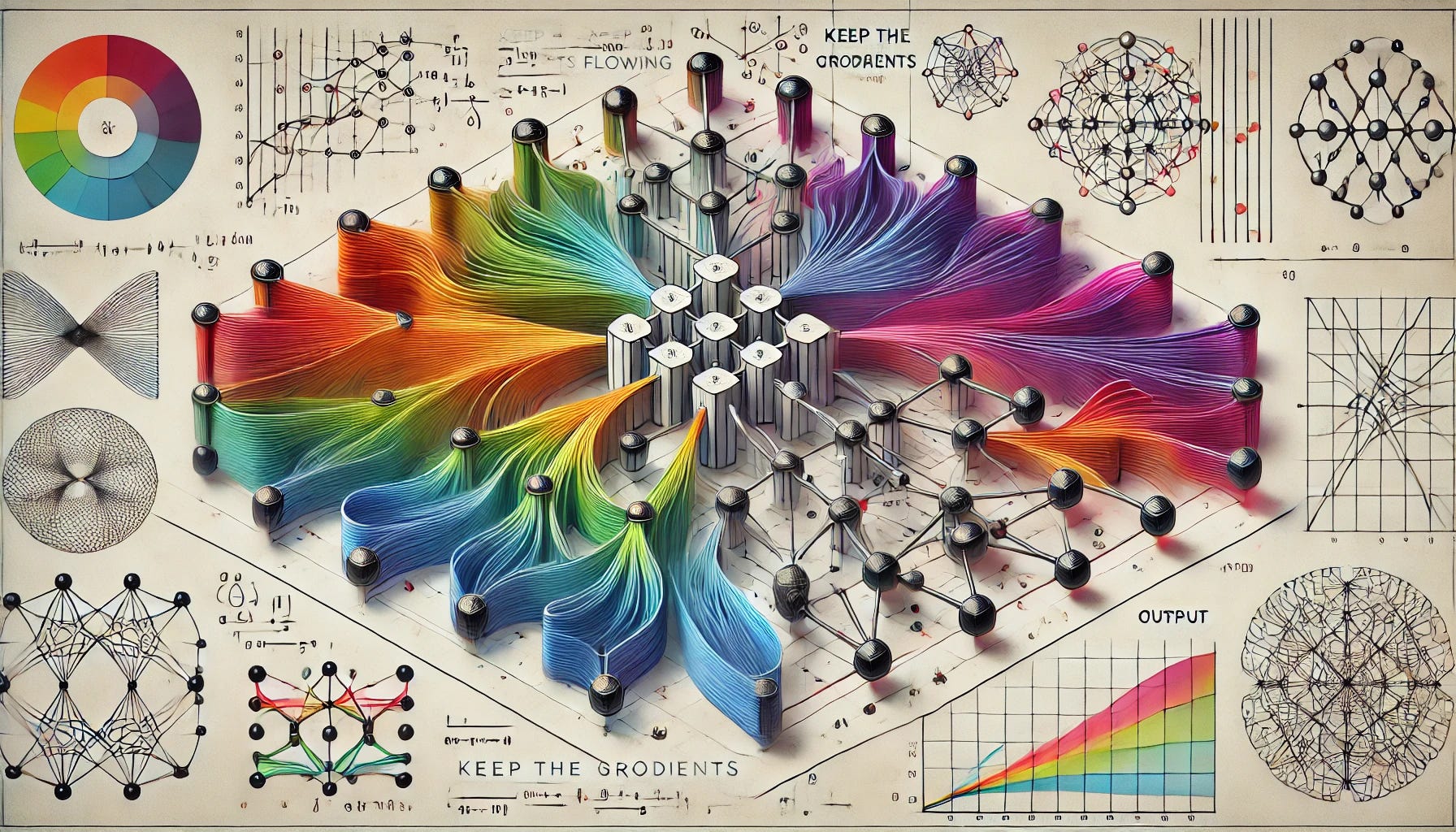 AI Image generated depicting the gradients flowing in Neural Networks
In recent years, the AI field has been obsessed with building larger and larger neural networks, believing that more complexity leads to better performance. Indeed, this approach has yielded incredible results, leading to breakthroughs in image recognition, language translation, and countless other areas.
But there's a catch. Just like a massive, overly complex machine can be costly to build and maintain, these enormous neural networks require significant computational resources and time to train. They can be slow, demanding a lot of memory and power, making deploying them on devices with limited resources challenging. Plus, they often become prone to "memorizing" the training data rather than truly understanding the underlying patterns, leading to poor performance on unseen data.
Sparse neural networks have partly solved the problem above. Think of sparse NNs as a leaner version of classic NNs. They carefully remove unnecessary parts and connections, resulting in a more efficient and leaner model that still maintains its power. They can train faster, require less memory, and are often more robust to noisy data.
However, training these sparse networks has been surprisingly difficult. Researchers have struggled to get them to perform as well as their larger, denser counterparts.
The paper we'll be exploring today - Keep the gradients flowing: Using gradient flow to study sparse network optimization by Tessera et al. - offers a fresh perspective on this challenge, taking a deep look at how these sparse networks learn and identifying critical aspects that hinder their training. By focusing on the flow of information within the network, represented by something called "gradient flow ," the researchers show what makes training sparse networks difficult and propose new techniques for optimization.
Think of it as uncovering the hidden wiring diagrams of the streamlined machine, and understanding how the remaining parts work together. By revealing the intricacies of gradient flow, we can fine-tune the training process and enable these leaner, more efficient neural networks to reach their full potential. Prepare to be amazed as we unpack the secrets of sparse network optimization!
Gradient Flow in Neural Networks
Every neural network, whether it's a giant, complex model or a streamlined, sparse one, learns by adjusting its connections (weights) to better fit the data. This process of learning is guided by the concept of gradient flow. Think of it as a compass that points the network in the right direction to minimize errors and improve accuracy.
But what exactly is gradient flow? In essence, it quantifies how much the network's error changes for its weights. The gradients themselves are essentially derivatives of the network's cost (error) function to its weights. The larger the gradient, the steeper the change in error, indicating that a small change in a particular weight will lead to a larger change in the error. This information is then used by the optimizer to update the weights, taking steps in the direction of lower error.
Let's clarify this with a simple analogy. Imagine you are hiking down a mountain in the fog. You don't know the exact path to the valley, but you want to reach the lowest point. Gradient flow acts like the slope of the mountain at your current location. If the slope is steep, you know that taking a step in that direction will lead you to a lower altitude quickly. Otherwise, if the slope is gentle, you'll have to take smaller steps.
In mathematical terms, the gradient flow (g_{fp}) at a particular point can be represented using the following formula:
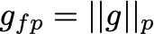 Gradient Flow at a particular point - Image by Author
where:
- g represents the gradient vector, which is a collection of all the gradients of the network's weights for the cost function (error). Essentially, it's a vector that points in the direction of the steepest ascent of the error function.
- || . ||p represents a norm, which essentially calculates the magnitude of the gradient vector. In the context of gradient flow, we are primarily interested in the strength or magnitude of the gradient, not necessarily its direction. Common norms include the L1 norm and the L2 norm.
So, the gradient flow gives us a sense of the strength of the gradient, indicating the potential for significant change in error to the weights. Larger gradient flows generally imply larger potential changes in error for changes in weights, which can be useful information for the optimizer.
However, when it comes to sparse neural networks, this standard formula for gradient flow can be a bit misleading. This is because the standard gradient flow measure includes the gradients of all weights, even those that have been masked (set to zero) during training. These masked weights don't participate in the forward pass or the actual computation of the network, so their gradients don't provide useful information. Including them in the calculation can obscure the true picture of how information flows through the active connections in the sparse network.
The researchers addressed this issue with a new metric called Effective Gradient Flow (EGF) , which provides a more insightful and accurate representation of gradient flow within sparse networks. This metric is central to the paper's findings and its contribution to understanding and optimizing sparse networks.
Effective Gradient Flow (EGF)
EGF is designed to provide a more accurate reflection of how information flows through the active connections in sparse networks. It achieves this by focusing solely on the gradients of the non-zero weights. It's like focusing the compass on the relevant parts of the mountain, ignoring the areas that are not part of the path you are currently following.
First, we calculate the masked gradient vector (g) for each layer:
 Masked gradient vector Formula - Image by Author
where:
- ∂𝐶/∂𝜃_l represents the gradient vector for layer l, **** containing the gradients of all weights in that layer for the cost function (C**)**.
- m_l is a binary mask for layer l , where a value of 1 indicates an active weight and a value of 0 indicates a masked (inactive) weight. The element-wise product (⊙) ensures that only the gradients of active weights are considered.
Then, the EGF is calculated as the average masked gradient norm across all layers:
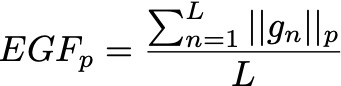 EGF Formula - Image by Author
where:
- ||g_n||_p represents the chosen norm (e.g., L1 or L2) of the masked gradient vector (g_n) for layer n.
- L is the total number of layers in the network.
Essentially, EGF takes the average magnitude of the gradients of active weights across all layers. This provides a much more meaningful representation of the flow of information within the active connections of a sparse network.
Benefits of EGF
EGF offers several significant advantages over the standard gradient flow measure, particularly in the context of sparse networks:
- Focuses on Active Connections: By incorporating the binary mask (m_l), EGF ensures that only the gradients of active weights are considered. This directly addresses the issue of misleading gradients from masked weights in standard gradient flow.
- Even Distribution Across Layers: EGF computes the average gradient norm across layers, preventing layers with a larger number of weights from disproportionately influencing the overall measure. This ensures that gradient flow is evaluated fairly across all layers, providing a more balanced view of the network's training dynamics.
- Stronger Correlation with Performance: The researchers empirically demonstrate that EGF consistently has a higher correlation with performance metrics like accuracy and loss, compared to standard gradient flow measures when used with sparse networks. This implies that EGF is a more reliable indicator of how well a sparse network is learning.
By providing a more accurate and insightful view of gradient flow, EGF helps us better understand the training dynamics of sparse networks. It allows us to pinpoint areas where the flow of information might be hindered and ultimately leads to a better understanding of how to optimize these lean and efficient models.
Same Capacity Sparse vs. Dense Comparison (SC-SDC)
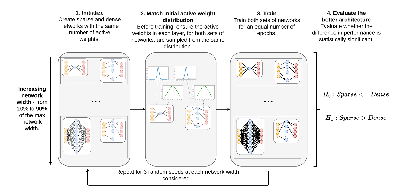 SameCapacity Sparse vs Dense Comparison (SC-SDC) - Image extracted from the original research paper (arXiv:2102.01670)
When evaluating the performance of sparse networks, it's crucial to compare them to their dense counterparts in a way that isolates the impact of sparsity. This is where the Same Capacity Sparse vs. Dense Comparison (SC-SDC) framework comes into play.
Traditional approaches to comparing sparse and dense networks often involve contrasting a sparse network with fewer parameters with a dense network with a larger number of parameters. While this might seem intuitive, it can lead to biased results. It's like comparing a small, efficient car to a large, luxurious SUV and concluding that the SUV is better simply because it has more features and a larger engine. The difference in performance might be due to the size difference, not necessarily the fundamental characteristics of the two types of vehicles.
SC-SDC tackles this issue by ensuring a truly fair comparison. It focuses on comparing sparse and dense networks with the same number of active connections and the same depth (number of layers). This ensures that any performance difference observed can be attributed directly to the presence or absence of connections, rather than differences in overall model capacity.
For each layer of the dense network, the corresponding layer in the sparse network is designed to have the same number of active weights. This means that the sparse network may have a larger total number of weights but only a subset of them are active during the training process.
Both the sparse and dense networks have the same number of layers (depth). This ensures that the fundamental structure and information processing pathways are similar between the two networks.
The active weights in both the sparse and dense networks are initialized using the same distribution. This guarantees that any performance differences are not simply due to differences in initial conditions.
To achieve the same capacity, the researchers in the paper use a process of masking. They randomly select a subset of weights to be active (non-zero) in the sparse network, ensuring that the number of active weights in each layer of the sparse network matches the number of weights in the corresponding layer of the dense network.
Benefits of SC-SDC
SC-SDC provides a powerful tool for understanding the optimization dynamics of sparse networks. Creating a level playing field, allows researchers to isolate the effects of sparsity and examine how different optimization and regularization strategies impact performance.
- Isolates the Impact of Sparsity: It enables us to understand how the mere presence or absence of connections affects a neural network's ability to learn and generalize.
- Provides a Fair Performance Benchmark: SC-SDC allows us to directly compare the performance of sparse and dense networks under identical conditions, helping us determine if sparsity is indeed beneficial for a particular task and architecture.
- Facilitates Exploration of Optimization Strategies: SC-SDC allows researchers to explore various optimization techniques specifically for sparse networks and examine how they affect training dynamics and overall performance.
How Architectural Choices and Training Strategies Impact Sparse Networks
The authors explored a wide range of architectural and training choices, including different activation functions, regularization techniques, and optimizers. Let's explore some of their key findings:
Batch Normalization
Batch Normalization (BatchNorm) is a technique designed to improve the training of deep neural networks by normalizing the inputs to each layer. This helps to mitigate issues like internal covariate shift - the change in the distribution of network activations due to the updating of parameters during training - which can slow down learning and make optimization more difficult.
Consider a mini-batch of activations from a particular layer, denoted as x1,x2,...,xm, where m is the number of samples in the mini-batch. BatchNorm normalizes these activations using the following steps:
Compute the Mini-Batch Mean The mean μB of the mini-batch activations is calculated as:
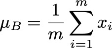 Mini-Batch mean Formula - Image by Author
This equation sums all the activations in the mini-batch and divides them by the number of activations to find their average value. Computing the mean centers the data around zero, which is essential for normalization.
Compute the Mini-Batch Variance The variance σ_B² measures how much the activations vary around the mean:
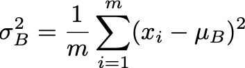 Mini-Batch Variance Formula - Image by Author
For each activation x_i , we subtract the mean μB to find its deviation from the mean, square this deviation to ensure it's positive, and then average these squared deviations over all activations. The variance quantifies the spread or dispersion of the activations.
Normalize the Activations Each activation x_i is then normalized to produce x^i :
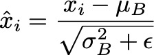 Activation Normalization Formula - Image by Author
In this equation, ϵ is a small constant (like 10^{-5}) added to the variance to prevent division by zero and improve numerical stability. By subtracting the mean and dividing by the standard deviation (the square root of the variance), we transform the activations to have a mean of zero and a variance of one. This standardization ensures that the scale of the activations remains consistent across layers and during training.
Scale and Shift Finally, we apply a linear transformation to the normalized activations:
 Scale and Shift Formula - Image by Author
Here, γ and β are learnable parameters that allow the network to restore the original distribution of activations if necessary. γ scales the normalized activation, and β shifts it. This step provides the network with the flexibility to adjust the normalized activations, which can improve its representational capacity.
In the context of sparse networks - networks where many weights are set to zero, reducing the number of active connections - BatchNorm is particularly beneficial:
- Stabilizes Gradient Flow : By normalizing the inputs to each layer, BatchNorm ensures that small changes in the weights don't lead to large changes in the activations. This helps prevent gradients from becoming too small (vanishing gradients) or too large (exploding gradients), which is crucial for effective learning.
- Improves Training Efficiency : Normalized activations allow the use of higher learning rates and reduce sensitivity to the initialization of weights. This is especially important in sparse networks, where the reduced number of connections can make the network more fragile during training.
The Sensitivity of EWMA Optimizers to High Gradient Flow
The paper investigates how different optimizers perform in the context of sparse networks, focusing on those that use an Exponentially Weighted Moving Average (EWMA) of past gradients, such as Adam and RMSProp. These optimizers adapt the learning rates based on the historical behavior of gradients, which can make them sensitive to high gradient flows.
Let's delve deeper into how these optimizers work, using the Adam optimizer as an example.
Adam Optimizer
Compute Gradients At each time step t , we compute the gradients of the loss function L_t for the parameters θ :
 Gradients Formula - Image by Author
Here, ∇θLt(θt−1) represents the vector of partial derivatives of the loss to each parameter in θ , evaluated at the previous parameter values θt−1.
Update Biased First Moment Estimate ( m_t ) The first-moment estimate mtm_tmt is an EWMA of the gradients:
 First moment Estimate Formula - Image by Author
- In this equation:
- β1 is the decay rate for the moving average of the gradients, typically set to a value like 0.90.90.9.
- m_{t-1} is the previous first-moment estimate (essentially the running average of past gradients).
- g_t is the current gradient.
- The term β1mt−1 gives weight to past gradients, while (1−β1)gt emphasizes the current gradient.
Update Biased Second Moment Estimate ( v_t ) The second-moment estimate v_t is an EWMA of the squared gradients:
 Second Moment Estimate - Image by Author
Here:
- β2 is the decay rate for the moving average of the squared gradients, typically set to a value like 0.999.
- g_t² denotes the element-wise square of the gradient vector g_t , capturing the variance of the gradients.
Compute Bias-Corrected Estimates Since mtm_tmt and v_t are initialized at zero, they are biased towards zero, especially in the initial time steps. To correct this bias, we compute:
 Bias-Corrected Estimates - Image by Author
The terms 1−β1 and 1−β2 adjust the estimates based on how many time steps have occurred. As t increases, β1 and β2 approach zero, reducing the bias in m_t and v_t.
Update Parameters Finally, we update the parameters θ :
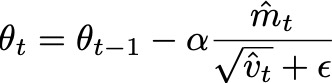 Parameters Update - Image by Author
Here:
- α is the learning rate.
- ϵ is a small constant (e.g., 10^{-8}) added to prevent division by zero.
- The fraction component on the right scales the update step based on the estimated first and second moments of the gradients. This allows for adaptive learning rates for each parameter.
When gradients are large (high gradient flow), EWMA optimizers can exhibit instability due to:
- Inflated Second Moment Estimate (v_t) : High gradients lead to large g²_t values, which can cause v_t to become large. Since v_t appears in the denominator when updating the parameters, a large v_t reduces the size of the parameter updates, effectively decreasing the learning rate.
- Delayed Adaptation : The moving averages m_t and v_t may not adapt quickly enough to sudden changes in gradient magnitudes, especially if β1 and β2 are close to 1. This can cause the optimizer to respond slowly to changes, leading to oscillations or divergence.
- Sensitivity to Regularization : When techniques like L2 regularization are used, they add additional terms to the gradients, increasing their magnitude and exacerbating the issues above.
L2 Regularization
L2 Regularization (also known as weight decay) adds a penalty to the loss function proportional to the square of the magnitude of the weights:
 L2 Regularization - Image by Author
Here:
- L0(θ) is the original loss function.
- λ is the regularization strength (a hyperparameter).
- ∣∣θ∣∣² is the squared Euclidean norm of the weight vector θ , calculated as ∣∣θ∣∣² = ∑_i θ².
The gradient of the regularized loss for θ is:
 Gradient with L2 Regularization - Image by Author
The term λθ increases the magnitude of the gradients, potentially leading to higher gradient flows.
In sparse networks, due to the combination of L2 regularization and fewer active parameters (weights), the gradients can be larger in magnitude. This is because the regularization term λθ adds a component proportional to the weights, and in sparse networks, the remaining weights might carry more significance.
Additionally, the sensitivity of EWMA optimizers like Adam and RMSProp to high gradients can cause instability, slow convergence, or even divergence during training. The inflated v_t can lead to excessively small parameter updates, hindering learning.
Optimizers that do not rely on EWMA of past gradients, such as Stochastic Gradient Descent (SGD) or Adagrad , may perform better in these situations because they are less sensitive to sudden changes in gradient magnitudes.
The Potential of Non-Sparse Activation Functions
The paper also explored the impact of different activation functions on the performance of sparse networks. Traditionally, ReLU (Rectified Linear Unit) has been a popular choice due to its simplicity and ability to mitigate the vanishing gradient problem. However, the researchers explored other activation functions, such as Swish and PReLU.
They discovered that these non-sparse activation functions, which don't inherently produce zero gradients, can be beneficial for sparse networks. This is particularly true for Swish, which has a non-monotonic behavior. Swish allows for the flow of negative gradients, which can contribute to better gradient flow and ultimately enhance the training process.
ReLU (Rectified Linear Unit)
The ReLU activation function is defined as:
 ReLU Formula - Image by Author
Its derivative, which is essential for backpropagation, is:
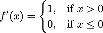 ReLU Derivative - Image by Author
For inputs x≤0 , the output is zero, introducing sparsity in the activations. If a neuron gets stuck with negative inputs, it may stop learning because the gradient f′(x) is zero, preventing weight updates. This phenomenon is known as the "dying ReLU" problem.
Swish Activation Function
The Swish activation function is defined as:
 Swish Formula - Image by Author
Where σ(βx) is the sigmoid function:
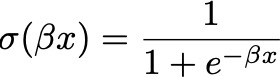 Sigmoid Function Formula - Image by Author
The derivative of Swish can be derived using the product rule of differentiation:
 Swish Derivative - Image by Author
The term σ(βx) represents the contribution from the linear part x. The term βx⋅σ(βx)(1−σ(βx)) comes from differentiating the sigmoid function.
Swish is not strictly increasing or decreasing, which can help in learning complex patterns. Unlike ReLU, Swish is smooth and differentiable everywhere, which can facilitate optimization. Even for negative x , the gradient f′(x) is non-zero, allowing for continued learning.
PReLU (Parametric ReLU)
PReLU introduces a learnable parameter aaa to control the slope for negative inputs:
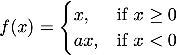 PReLU Formula - Image by Author
The derivative is:
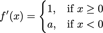 PReLU derivative - Image by Author
The parameter aaa (typically a small positive value) allows the activation function to have a small, non-zero gradient when x <0. This prevents the neuron from dying, as it can still update its weights even when the input is negative.
The parameter a is learned during training, allowing the network to adjust the activation function based on the data. With a >0, the gradient for negative inputs is non-zero, preventing neurons from becoming inactive.
In sparse networks, using activation functions that allow for non-zero gradients even when the input is negative can be particularly beneficial. Non-sparse activation functions like Swish and PReLU ensures that neurons continue to learn even when they receive negative inputs, due to non-zero gradients.
By preventing gradients from becoming zero, these activation functions facilitate better propagation of error signals during backpropagation, enhancing the learning process.
Also, neurons are less likely to become inactive permanently, as can happen with ReLU when weights update in such a way that the neuron only receives negative inputs.
Results
The results from these experiments highlight several important points:
Gradient flow is a critical factor in the training of sparse networks. Understanding and controlling gradient flow is crucial for achieving good performance.
BatchNorm is particularly beneficial for sparse networks, helping to stabilize the training process.
EWMA optimizers can be problematic when used with certain regularization techniques or data augmentation strategies. This is due to their sensitivity to high gradient flow.
Non-sparse activation functions can improve the performance of sparse networks. This can be attributed to their ability to facilitate a more stable and informative gradient flow.
The Role of Initialization
One of the most important takeaways from this research is that initialization is just one piece of the puzzle when it comes to optimizing sparse networks. Traditionally, a lot of research focused on finding optimal weight initialization strategies for sparse networks. However, the paper reveals that other factors, like optimization algorithms, activation functions, and regularization techniques, play a crucial role in determining the performance of sparse networks.
This broader perspective emphasizes the need to reconsider many of the default choices made when training neural networks, especially in the context of sparse networks. We can no longer simply assume that optimization strategies developed for dense networks will be equally effective for sparse networks.
The Importance of Stable Gradient Flow
Understanding gradient flow is essential when training neural networks, especially sparse ones. In simple terms, gradient flow refers to how gradients - the signals used to update the network's weights during training - propagate through the layers of a neural network. The paper emphasizes that achieving a stable and informative gradient flow is crucial for the successful training of sparse networks. When the gradient flow is stable, the network can effectively update its weights, learn from the data, and improve its performance over time.
This insight opens up exciting avenues for future research. By focusing on developing new regularization techniques or normalization methods that promote stable gradient flow specifically in sparse networks, we can enhance their learning capabilities. This could involve modifying existing methods or creating entirely new approaches tailored to address the unique challenges posed by sparsity in neural networks.
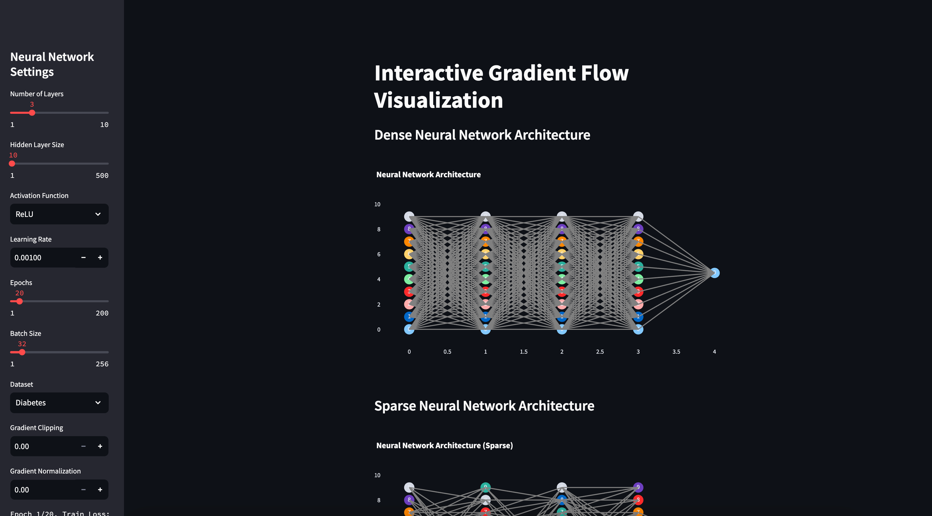 Screenshot of Gradient Flow Visualizer Web App — Built by Author
To help you see firsthand how different components affect both the training process and gradient flow in dense and sparse neural networks, I've built a web app, which allows you to train neural networks with configurations that you customize, giving you a hands-on understanding of these concepts. You can specify parameters such as the number of hidden layers in the model and the number of nodes in each hidden layer. The app lets you choose the activation function used after each layer, offering options like ReLU, PReLU, Swish, and Sigmoid. You can set the learning rate, determine how many epochs (iterations) you want the model to train over, and select the batch size for training. Additionally, the app provides datasets from the sci-kit-learn library for you to work with. For regression tasks, you can choose the "Diabetes" dataset, and for classification tasks, options include the "Iris," "Wine," and "Breast Cancer" datasets. There's also the option to apply techniques like gradient clipping and gradient normalization to further experiment with training dynamics.
The app is free to use, and the code is available here:
GitHub - cristianleoo/gradient-flow-optimizer-neural-networks
You may be able to access the website here:
However, streamlit - the hosting platform - may temporarily bring it down. If that happens don't hesitate to reach out to me and I will bring it up again. If you want to self-host it, you can follow the guide in GitHub repo.
Now, back to the app. Once you've set up your desired configuration, the app creates both dense and sparse neural network models based on your settings and trains them on the selected dataset. During training, it collects data on gradient flow, loss, and various performance metrics, allowing you to observe how different factors influence the learning process.
For example, if you configure a dense neural network with three hidden layers and ten nodes per layer, the app visualizes this architecture for you.
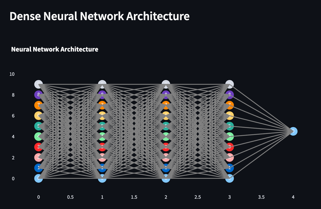 Example of a Dense Neural Network architecture with 3 hidden layers and 10 nodes per layer - Image by Author
The app will also generate a train a sparse neural network with the same structural parameters, you'll see how sparsity changes the architecture. These visual representations help you understand the structural differences between dense and sparse networks.
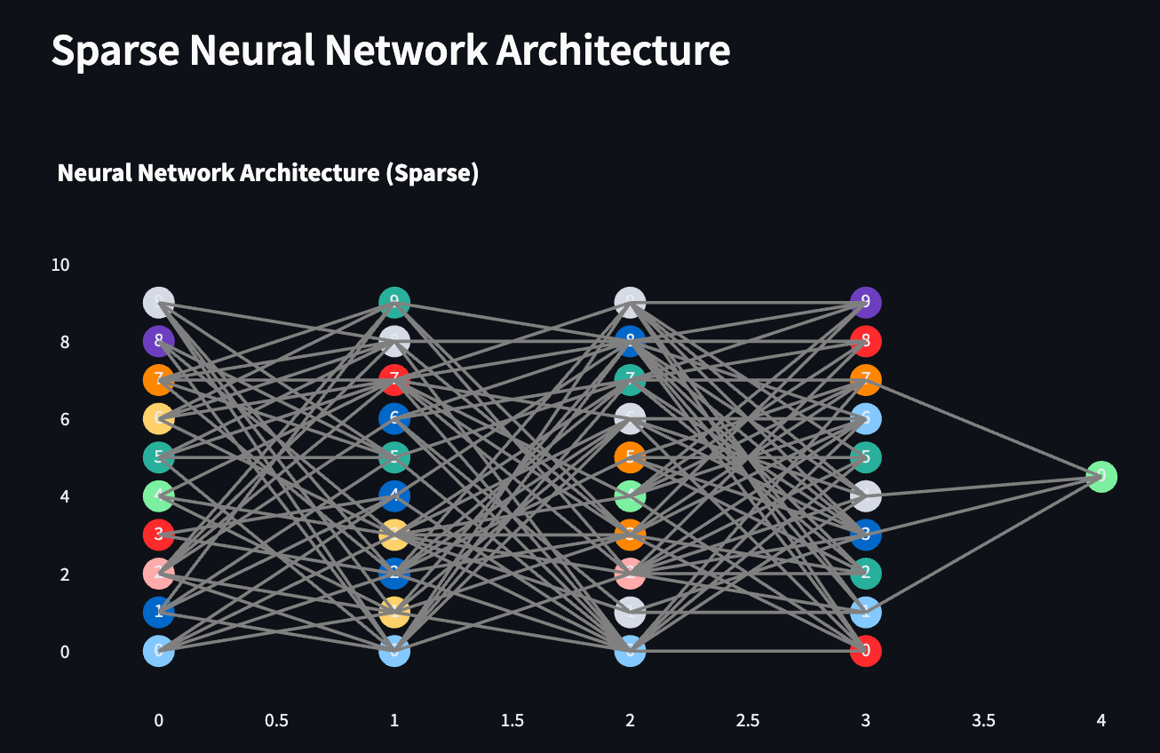 Example of a Sparse Neural Network architecture with 3 hidden layers and 10 nodes per layer - Image by Author
After the training is completed, the app provides a range of visualizations and statistics to help you delve deeper into gradient flow and model performance. For both dense and sparse models, it plots metrics over time, such as loss, accuracy, precision, recall, and F1 score. These graphs enable you to see how the models' performance evolves throughout the training process, giving you insights into their learning behaviors.
For instance, you might examine a plot of the Mean Squared Error (MSE) over 20 epochs of training, which illustrates how the error decreases as the model learns. This can show you how quickly the model is converging and whether it's learning effectively from the data.
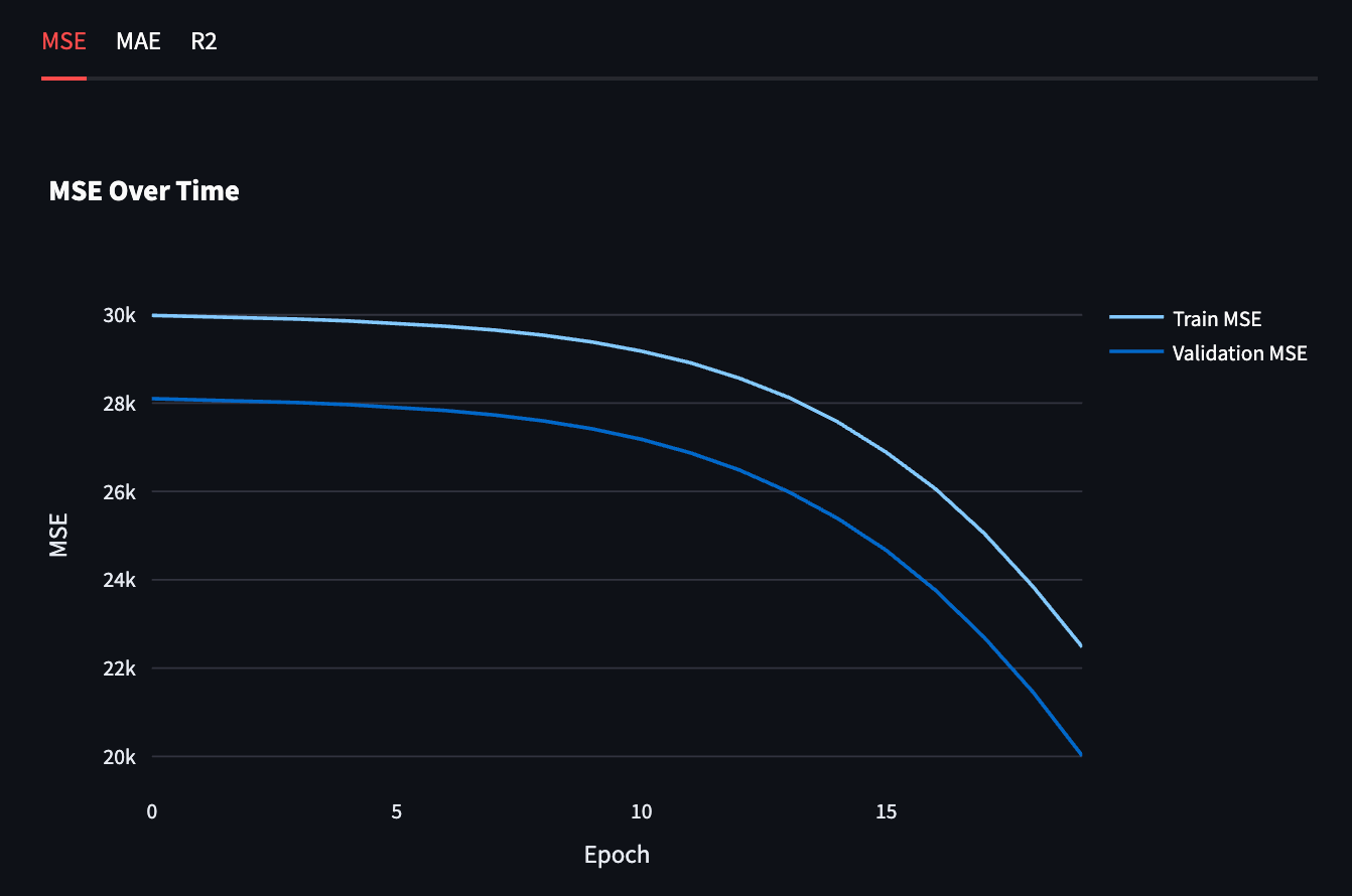 MSE plot for NN training over 20 epochs - Image by Author
The app also provides visualizations of gradient flow distribution, such as boxplots that display the distribution of gradient norms across the different layers of the network. These plots help you identify potential issues like vanishing or exploding gradients by highlighting how the gradients vary throughout the network. By examining these visualizations, you can see whether the gradients are consistently flowing through all layers or if they're diminishing or amplifying in certain parts of the network.
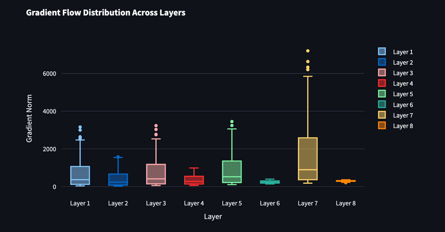 Gradient Flow Distribution Across Layers - Image by Author
Additionally, the app plots how the gradient norms for each layer change over time during training. This allows you to observe trends and spot any potential instabilities in the gradient flow as the model learns. For example, you might notice that the gradients in the earlier layers are gradually decreasing, which could indicate the vanishing gradient problem. Alternatively, if the gradients are increasing uncontrollably, it might signal exploding gradients.
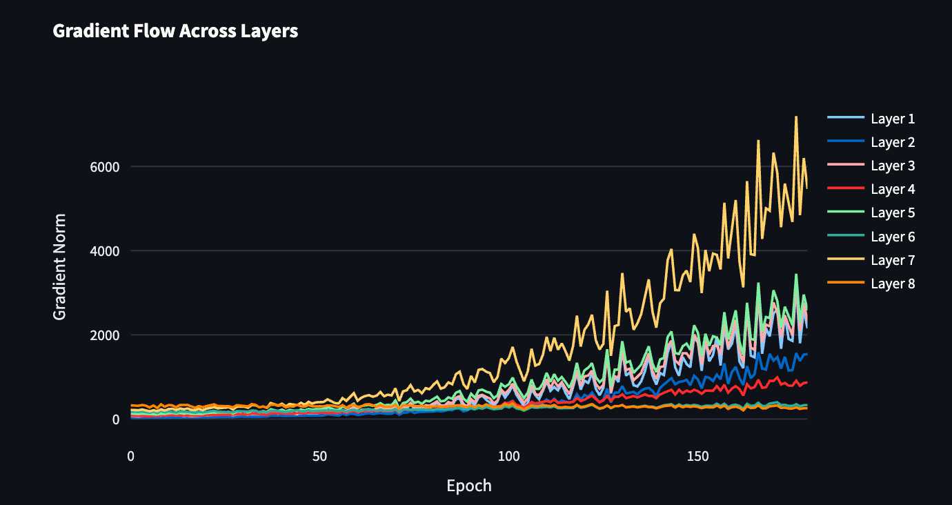 Gradient Flow Across Layers - Image by Author
Moreover, the app provides detailed statistics for each layer, including initial and final gradient values, the mean and standard deviation of the gradients, and percentile information. It also reports the number of vanishing gradients (very small gradients that may hinder learning) and exploding gradients (very large gradients that can cause instability). These statistics give you quantitative measures to assess the health of your network's training process.
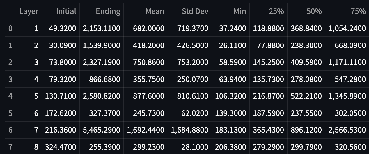 Stats table for gradients across layers - Image by Author
Interpreting these results is key to understanding and improving your models. A stable gradient flow is characterized by consistent, non-zero gradient norms across layers and over time. When examining the gradient flow distribution plots, look for relatively uniform distributions, indicating that gradients are properly propagating through the network. In the gradient flow over time plots, smooth and steady lines suggest that the gradients are stable, which is desirable for effective learning.
If you observe very small gradient norms, especially in the earlier layers of the network, this could point to the vanishing gradient problem. In this scenario, the gradients are too small to make meaningful updates to the weights, hindering the network's ability to learn from the data. Conversely, extremely large gradient norms might indicate exploding gradients, where the updates become so large that they destabilize the training process. Both situations can be identified through the visualizations and statistics provided by the app.
By experimenting with different activation functions, learning rates, and other parameters, you can assess their impact on gradient flow. For instance, you might find that using the Swish activation function leads to a more stable gradient flow compared to ReLU in a sparse network. Comparing the results between dense and sparse networks also helps you understand how sparsity affects the flow of information. You might observe that sparse networks are more susceptible to vanishing gradients, emphasizing the importance of careful configuration and potentially the use of techniques like Batch Normalization or alternative activation functions to mitigate this issue.
Conclusion
The research highlighted the importance of gradient flow, the need for a broader perspective on sparse network optimization, and the potential for tailored optimization strategies. By embracing a more nuanced understanding of gradient flow and carefully considering architectural choices and training strategies, we can better understand what's happening behind this "black-box" architecture.
This exploration is just the beginning. As the field of deep learning continues to evolve, the ideas presented in "Keep the Gradients Flowing" will undoubtedly shape the future of sparse network optimization. Master the math I provided in this article, clone the repo from GitHub, make the code your own, and contribute to the research of gradient flow optimization!
References
- Tessera et al. (2021). Keep the Gradients Flowing: Using Gradient Flow to Study Sparse Network Optimization. arXiv:2102.01670. Retrieved from https://arxiv.org/abs/2102.01670.
- Kingma, D.P., & Ba, J. (2015). Adam: A Method for Stochastic Optimization. arXiv:1412.6980. Retrieved from https://arxiv.org/abs/1412.6980.
- Ioffe, S., & Szegedy, C. (2015). Batch Normalization: Accelerating Deep Network Training by Reducing Internal Covariate Shift. In Proceedings of the 32nd International Conference on Machine Learning (ICML). pp. 448–456.
- Ramachandran, P., Zoph, B., & Le, Q.V. (2017). Searching for Activation Functions. arXiv:1710.05941. Retrieved from https://arxiv.org/abs/1710.05941.
- Srivastava, N., Hinton, G., Krizhevsky, A., Sutskever, I., & Salakhutdinov, R. (2014). Dropout: A Simple Way to Prevent Neural Networks from Overfitting. Journal of Machine Learning Research , 15(1), 1929–1958.
- Nair, V., & Hinton, G.E. (2010). Rectified Linear Units Improve Restricted Boltzmann Machines. In Proceedings of the 27th International Conference on Machine Learning (ICML).
- Paszke, A., et al. (2019). PyTorch: An Imperative Style, High-Performance Deep Learning Library. In Advances in Neural Information Processing Systems (NeurIPS). pp. 8024–8035.
Register Now to Continue Reading
Unlock Towards Data Science with a Free Account
All articles on Towards Data Science are available to registered users. Create a free account today to access this article and thousands more.
Register for freeSign in to your account
 Written By
See all from Cristian Leo
Artificial IntelligenceData ScienceDeep LearningMachine LearningMathematics
Share This Article
Towards Data Science is a community publication. Submit your insights to reach our global audience and earn through the TDS Author Payment Program.
Write for TDS
Related Articles
Machine Learning
Evidence that proves why bagging algorithms like random forest perform better than decision tree
Jason Chong
May 2, 20226 min read
Artificial Intelligence
Cleaner Code and Fewer Loops? Count me in.
Dario Radečić
March 14, 20204 min read
Artificial Intelligence
Avoid the mistake of overfitting and underfitting
NVS Yashwanth
September 21, 20204 min read
Data Science
A fun introduction to GLMs using an Olympics dataset
Jamshaid Shahir, Ph.D
August 6, 202110 min read
Deep Learning
Bootstrap Your Own Latent: A New Approach to Self-Supervised Learning by J. Grill et. al.
Sascha Kirch
September 7, 202310 min read
Deep Learning
A journey of tooling decisions
Tobias Petri
September 28, 202011 min read
Artificial Intelligence
An Interactive Guide to Optimizing and Tuning Hyperparameters
Will Badr
August 6, 20195 min read
Artificial Intelligence
Build a portfolio and become job-ready as you learn
Sharan Kumar Ravindran
September 19, 202112 min read
Artificial Intelligence
Key Driver Analysis with PowerBI
Deepak Verma
January 10, 20215 min read
Your home for data science and AI. The world's leading publication for data science, data analytics, data engineering, machine learning, and artificial intelligence professionals.
Subscribe to Our NewsletterWrite For TDS•About•Advertise•Privacy Policy•Terms of Use
© Insight Media Group, LLC 2026•The New Stack•roadmap.sh•Creator Network