保留正文与补采附件。源页面当前未重新核验;具体限制见交付清单。
 We value your privacy
We use cookies to enhance your browsing experience, serve personalised ads or content, and analyse our traffic. By clicking "Accept All", you consent to our use of cookies.
Customise Reject All Accept All
Customise Consent Preferences
 We use cookies to help you navigate efficiently and perform certain functions. You will find detailed information about all cookies under each consent category below.
The cookies that are categorised as "Necessary" are stored on your browser as they are essential for enabling the basic functionalities of the site. ... Show more
NecessaryAlways Active
Necessary cookies are required to enable the basic features of this site, such as providing secure log-in or adjusting your consent preferences. These cookies do not store any personally identifiable data.
-
Cookie
BCTempID
-
Duration
10 minutes
-
Description
No description available.
-
Cookie
__cf_bm
-
Duration
1 hour
-
Description
This cookie, set by Cloudflare, is used to support Cloudflare Bot Management.
-
Cookie
AWSALBCORS
-
Duration
7 days
-
Description
Amazon Web Services set this cookie for load balancing.
-
Cookie
_cfuvid
-
Duration
session
-
Description
Cloudflare sets this cookie to track users across sessions to optimize user experience by maintaining session consistency and providing personalized services
-
Cookie
li_gc
-
Duration
6 months
-
Description
Linkedin set this cookie for storing visitor's consent regarding using cookies for non-essential purposes.
-
Cookie
__hssrc
-
Duration
session
-
Description
This cookie is set by Hubspot whenever it changes the session cookie. The __hssrc cookie set to 1 indicates that the user has restarted the browser, and if the cookie does not exist, it is assumed to be a new session.
-
Cookie
__hssc
-
Duration
1 hour
-
Description
HubSpot sets this cookie to keep track of sessions and to determine if HubSpot should increment the session number and timestamps in the __hstc cookie.
-
Cookie
wpEmojiSettingsSupports
-
Duration
session
-
Description
WordPress sets this cookie when a user interacts with emojis on a WordPress site. It helps determine if the user's browser can display emojis properly.
-
Cookie
BCSessionID
-
Duration
1 year 1 month 4 days
-
Description
Blueconic sets this cookie as a unique identifier for the BlueConic profile.
-
Cookie
_octo
-
Duration
1 year
-
Description
No description available.
-
Cookie
logged_in
-
Duration
1 year
-
Description
No description available.
-
Cookie
__Secure-YEC
-
Duration
past
-
Description
YouTube sets this cookie to stores the user's video player preferences using embedded YouTube video
-
Cookie
__eoi
-
Duration
6 months
-
Description
Description is currently not available.
-
Cookie
AWSALBTGCORS
-
Duration
7 days
-
Description
No description available.
-
Cookie
login-status-p
-
Duration
past
-
Description
Description is currently not available.
-
Cookie
AWSALBTG
-
Duration
7 days
-
Description
No description available.
-
Cookie
csrf_token
-
Duration
session
-
Description
No description available.
-
Cookie
token_v2
-
Duration
1 day
-
Description
Description is currently not available.
-
Cookie
D
-
Duration
1 year
-
Description
Description is currently not available.
-
Cookie
PHPSESSID
-
Duration
session
-
Description
This cookie is native to PHP applications. The cookie stores and identifies a user's unique session ID to manage user sessions on the website. The cookie is a session cookie and will be deleted when all the browser windows are closed.
-
Cookie
VISITOR_PRIVACY_METADATA
-
Duration
6 months
-
Description
YouTube sets this cookie to store the user's cookie consent state for the current domain.
-
Cookie
cookietest
-
Duration
session
-
Description
The cookietest cookie is typically used to determine whether the user's browser accepts cookies, essential for website functionality and user experience.
-
Cookie
__Host-airtable-session
-
Duration
1 year
-
Description
This cookie is used to enable us to integrate the services of Airtable.
-
Cookie
__Host-airtable-session.sig
-
Duration
1 year
-
Description
This cookie is used to enable us to integrate the services of Airtable.
-
Cookie
m
-
Duration
1 year 1 month 4 days
-
Description
Stripe sets this cookie for fraud prevention purposes. It identifies the device used to access the website, allowing the website to be formatted accordingly.
-
Cookie
BIGipServer*
-
Duration
session
-
Description
Marketo sets this cookie to collect information about the user's online activity and build a profile about their interests to provide advertisements relevant to the user.
-
Cookie
__cfruid
-
Duration
session
-
Description
Cloudflare sets this cookie to identify trusted web traffic.
-
Cookie
_GRECAPTCHA
-
Duration
6 months
-
Description
Google Recaptcha service sets this cookie to identify bots to protect the website against malicious spam attacks.
-
Cookie
__Secure-YNID
-
Duration
6 months
-
Description
Google cookie used to protect user security and prevent fraud, especially during the login process.
-
Cookie
cookieyes-consent
-
Duration
1 year
-
Description
CookieYes sets this cookie to remember users' consent preferences so that their preferences are respected on subsequent visits to this site. It does not collect or store any personal information about the site visitors.
Functional
Functional cookies help perform certain functionalities like sharing the content of the website on social media platforms, collecting feedback, and other third-party features.
-
Cookie
lidc
-
Duration
1 day
-
Description
LinkedIn sets the lidc cookie to facilitate data center selection.
-
Cookie
brw
-
Duration
1 year
-
Description
No description available.
-
Cookie
brwConsent
-
Duration
5 minutes
-
Description
Description is currently not available.
-
Cookie
WMF-Uniq
-
Duration
1 year
-
Description
Description is currently not available.
-
Cookie
loom_anon_comment
-
Duration
1 year
-
Description
No description available.
-
Cookie
loom_referral_video
-
Duration
session
-
Description
Description is currently not available.
-
Cookie
VISITOR_INFO1_LIVE
-
Duration
6 months
-
Description
A cookie set by YouTube to measure bandwidth that determines whether the user gets the new or old player interface.
-
Cookie
yt-remote-connected-devices
-
Duration
Never Expires
-
Description
YouTube sets this cookie to store the user's video preferences using embedded YouTube videos.
-
Cookie
ytidb::LAST_RESULT_ENTRY_KEY
-
Duration
Never Expires
-
Description
The cookie ytidb::LAST_RESULT_ENTRY_KEY is used by YouTube to store the last search result entry that was clicked by the user. This information is used to improve the user experience by providing more relevant search results in the future.
-
Cookie
yt-remote-device-id
-
Duration
Never Expires
-
Description
YouTube sets this cookie to store the user's video preferences using embedded YouTube videos.
-
Cookie
yt-remote-session-name
-
Duration
session
-
Description
The yt-remote-session-name cookie is used by YouTube to store the user's video player preferences using embedded YouTube video.
-
Cookie
yt-remote-fast-check-period
-
Duration
session
-
Description
The yt-remote-fast-check-period cookie is used by YouTube to store the user's video player preferences for embedded YouTube videos.
-
Cookie
yt-remote-session-app
-
Duration
session
-
Description
The yt-remote-session-app cookie is used by YouTube to store user preferences and information about the interface of the embedded YouTube video player.
-
Cookie
yt-remote-cast-available
-
Duration
session
-
Description
The yt-remote-cast-available cookie is used to store the user's preferences regarding whether casting is available on their YouTube video player.
-
Cookie
yt-remote-cast-installed
-
Duration
session
-
Description
The yt-remote-cast-installed cookie is used to store the user's video player preferences using embedded YouTube video.
-
Cookie
cp_session
-
Duration
3 months
-
Description
Codepen sets this cookie for Help systems found in the website.
-
Cookie
loid
-
Duration
1 year 1 month 4 days
-
Description
This cookie is set by the Reddit. The cookie enables the sharing of content from the website onto the social media platform.
Analytics
Analytical cookies are used to understand how visitors interact with the website. These cookies help provide information on metrics such as the number of visitors, bounce rate, traffic source, etc.
-
Cookie
__hstc
-
Duration
6 months
-
Description
Hubspot set this main cookie for tracking visitors. It contains the domain, initial timestamp (first visit), last timestamp (last visit), current timestamp (this visit), and session number (increments for each subsequent session).
-
Cookie
hubspotutk
-
Duration
6 months
-
Description
HubSpot sets this cookie to keep track of the visitors to the website. This cookie is passed to HubSpot on form submission and used when deduplicating contacts.
-
Cookie
_ga
-
Duration
1 year 1 month 4 days
-
Description
Google Analytics sets this cookie to calculate visitor, session and campaign data and track site usage for the site's analytics report. The cookie stores information anonymously and assigns a randomly generated number to recognise unique visitors.
-
Cookie
ga*
-
Duration
1 year 1 month 4 days
-
Description
Google Analytics sets this cookie to store and count page views.
-
Cookie
__Host-psifi.analyticsTrace
-
Duration
6 hours
-
Description
Description is currently not available.
-
Cookie
__Host-psifi.analyticsTraceV2
-
Duration
6 hours
-
Description
Description is currently not available.
-
Cookie
_gh_sess
-
Duration
session
-
Description
GitHub sets this cookie for temporary application and framework state between pages like what step the user is on in a multiple step form.
-
Cookie
YSC
-
Duration
session
-
Description
YSC cookie is set by Youtube and is used to track the views of embedded videos on Youtube pages.
-
Cookie
ajs_anonymous_id
-
Duration
1 year
-
Description
This cookie is set by Segment to count the number of people who visit a certain site by tracking if they have visited before.
-
Cookie
vuid
-
Duration
1 year 1 month 4 days
-
Description
Vimeo installs this cookie to collect tracking information by setting a unique ID to embed videos on the website.
Performance
Performance cookies are used to understand and analyse the key performance indexes of the website which helps in delivering a better user experience for the visitors.
-
Cookie
AWSALB
-
Duration
7 days
-
Description
AWSALB is an application load balancer cookie set by Amazon Web Services to map the session to the target.
-
Cookie
acq
-
Duration
past
-
Description
Description is currently not available.
-
Cookie
acq.sig
-
Duration
past
-
Description
Description is currently not available.
-
Cookie
ptc
-
Duration
2 years
-
Description
No description available.
Advertisement
Advertisement cookies are used to provide visitors with customised advertisements based on the pages you visited previously and to analyse the effectiveness of the ad campaigns.
-
Cookie
muc_ads
-
Duration
1 year 1 month 4 days
-
Description
Twitter sets this cookie to collect user behaviour and interaction data to optimize the website.
-
Cookie
guest_id_marketing
-
Duration
1 year 1 month 4 days
-
Description
Twitter sets this cookie to identify and track the website visitor.
-
Cookie
guest_id_ads
-
Duration
1 year 1 month 4 days
-
Description
Twitter sets this cookie to identify and track the website visitor.
-
Cookie
personalization_id
-
Duration
1 year 1 month 4 days
-
Description
Twitter sets this cookie to integrate and share features for social media and also store information about how the user uses the website, for tracking and targeting.
-
Cookie
guest_id
-
Duration
1 year 1 month 4 days
-
Description
Twitter sets this cookie to identify and track the website visitor. It registers if a user is signed in to the Twitter platform and collects information about ad preferences.
-
Cookie
bcookie
-
Duration
1 year
-
Description
LinkedIn sets this cookie from LinkedIn share buttons and ad tags to recognize browser IDs.
-
Cookie
__Secure-ROLLOUT_TOKEN
-
Duration
6 months
-
Description
YouTube sets this cookie to manage feature rollout and experimentation. It helps Google control which new features or interface changes are shown to users as part of testing and staged rollouts, ensuring consistent experience for a given user during an experiment.
-
Cookie
yt.innertube::nextId
-
Duration
Never Expires
-
Description
YouTube sets this cookie to register a unique ID to store data on what videos from YouTube the user has seen.
-
Cookie
yt.innertube::requests
-
Duration
Never Expires
-
Description
YouTube sets this cookie to register a unique ID to store data on what videos from YouTube the user has seen.
-
Cookie
session_tracker
-
Duration
session
-
Description
This cookie is set by the Reddit. This cookie is used to identify trusted web traffic. It also helps in adverstising on the website.
-
Cookie
edgebucket
-
Duration
session
-
Description
Reddit sets this cookie to save the information about a log-on Reddit user, for the purpose of advertisement recommendations and updating the content.
-
Cookie
did
-
Duration
1 year
-
Description
Arbor sets this cookie to show targeted ads to site visitors.This cookie expires after 2 months or 1 year.
Uncategorised
Other uncategorised cookies are those that are being analysed and have not been classified into a category as yet.
No cookies to display.
Reject All Save My Preferences Accept All
Toggle SearchToggle Mobile Navigation
Publish AI, ML & data-science insights to a global community of data professionals.
Sign inSubmit an Article
LatestEditor's PicksNewsletterShipAI
Write For TDS
LinkedInXToggle Search
Deep Learning
The Math Behind Gated Recurrent Units
Dive into advanced deep learning with gated recurrent units (GRUs), understand their mathematics, and implement them from scratch.
Cristian Leo
June 4, 202429 min read
 Image generated by DALL-E
Gated Recurrent Units (GRUs) are a powerful type of recurrent neural network (RNN) designed to handle sequential data efficiently. In this article, we'll explore what GRUs are, and their math, and we will build an implementation from scratch in Python.
Learn this step by step with the interactive Machine Learning and Computer Science roadmaps.
Index
1: Understanding the Basics ∘ 1.1: What are GRUs? ∘ 1.2: Comparison with LSTMs and Vanilla RNNs 2: The Architecture of GRUs ∘ 2.1: GRU Cell Structure 3: The Mathematics of GRUs ∘ 3.1: Update Gate ∘ 3.2: Reset Gate ∘ 3.3: Candidate Activation ∘ 3.4: Step-by-Step Example 4: Building GRU From Scratch in Python ∘ 4.1: Imports and Custom Classes ∘ 4.2: GRU Class ∘ 4.3: GRUTrainer Class ∘ 4.4: TimeSeriesDataset Class ∘ 4.5: Training the GRU Model 5: Conclusion
1: Understanding the Basics
1.1: What are GRUs?
GRUs, or Gated Recurrent Units, are a type of recurrent neural network (RNN) introduced by Kyunghyun Cho and his colleagues in 2014. Think of GRUs as a smarter version of traditional RNNs, designed to handle sequences of data more effectively.
Imagine you're trying to learn a song by listening to it repeatedly. A basic RNN might forget the beginning of the song by the time it gets to the end. GRUs solve this problem by using gates that control what information is remembered and what is forgotten.
GRUs simplify the structure of Long Short-Term Memory (LSTM) networks by merging the input and forget gates into a single update gate and adding a reset gate. This makes them faster to train and easier to work with, while still keeping the ability to remember important information for a long time.
Update Gate : This gate decides how much of the past information should be carried forward to the future.
Reset Gate : This gate determines how much of the past information to forget.
These gates help GRUs maintain a balance between remembering important details and forgetting unimportant ones, similar to how you might focus on remembering the melody of a song while ignoring the background noise.
GRUs are great for tasks where data comes in sequences, like predicting the stock market, understanding language, or even generating music. They can learn patterns in data by keeping track of past information and using it to make better predictions. This makes them incredibly useful for any application where understanding the context from previous data points is crucial.
1.2: Comparison with LSTMs and Vanilla RNNs
To understand where GRUs fit in, let's compare them with LSTMs and Vanilla RNNs.
Vanilla RNNs Think of Vanilla RNNs as the basic version of recurrent neural networks. They work by passing information from one time step to the next, like a relay race where each runner passes the baton to the next. However, they have a big flaw: they tend to forget things over long sequences. This is due to the vanishing gradient problem, which makes it hard for them to learn long-term dependencies in data.
Here's my previous article about Recurrent Neural Networks, where we build them from scratch:
The Math Behind Recurrent Neural Networks
LSTMs Long Short-Term Memory Networks were designed to fix this problem. They use a more complex structure with three types of gates: input, forget, and output gates. These gates act like a sophisticated filing system, deciding what information to keep, what to update, and what to discard. This allows LSTMs to remember important information for long periods, making them great for tasks where context over many time steps is crucial, like understanding paragraphs of text or recognizing patterns in long time series.
Here's my previous article about LSTM:
The Math Behind LSTM
GRUs Gated Recurrent Units are a streamlined version of LSTMs. They simplify things by combining the input and forget gates into a single update gate, and they also have a reset gate. This makes GRUs less computationally intensive and faster to train than LSTMs, while still being able to handle long-term dependencies effectively.
2: The Architecture of GRUs
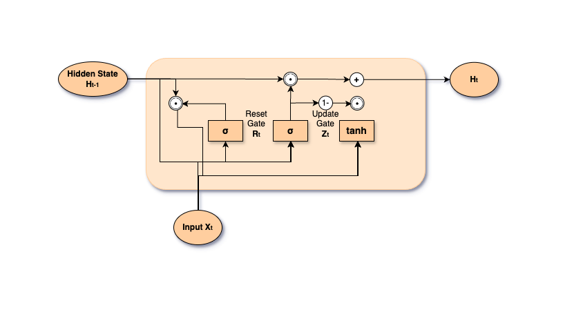 Gated Recurrent Unit Diagram - Image by Author
2.1: GRU Cell Structure
Now, let's take a look inside a single GRU cell. A GRU cell can be thought of as a small control unit in a factory that decides how much of the old information to keep and how much new information to add. It does this through two main components: the update gate and the reset gate. Let's explore these two concepts in more detail.
Update Gate: This gate acts like a smart filter. It determines how much of the past information should be carried forward. If the update gate decides a piece of information is important, it will keep it; otherwise, it will discard it.
Reset Gate: This gate decides how much of the past information to forget. When the reset gate is activated, it allows the cell to ignore parts of the past data, which helps in focusing on new, relevant information.
Each GRU cell takes in the current input and the previous hidden state (like a memory of what happened before). The update gate is calculated using the current input and the previous hidden state. This helps the cell decide how much of the past information to keep.
The reset gate is calculated similarly, using the current input and the previous hidden state. This gate helps decide how much of the past information to forget.
With the reset gate applied, a candidate for the new hidden state is created by combining the current input and the previous state. This candidate represents the potential new information that could be added to the hidden state.
The update gate then decides the final hidden state by blending the previous hidden state and the candidate activation. This blend ensures that important past information is retained while incorporating relevant new information.
3: The Mathematics of GRUs
In this section, we will go over the math behind GRU. I suggest you have the image at the top of the article displaying the GRU architecture, making it easier to see how the data flows and get transformed.
3.1: Update Gate
As we said before, the update gate determines how much of the past information should be carried forward to influence the current state. This gate helps the GRU retain important information over long sequences, making it effective for handling sequential data.
The update gate _z t is calculated using the current input _x t and the previous hidden state _h t −1. The formula for the update gate is:
 Update Gate Formula - Image by Author
Here:
- 𝑧_𝑡 i s the update gate at time step t.__
- 𝜎 is the sigmoid activation function, which squashes the output to be between 0 and 1.
- 𝑊_𝑧 is the weight matrix for the update gate.
- ℎ_𝑡−1 is the hidden state from the previous time step.
- 𝑥_𝑡 is the current input.
- [_h t−1, _x t] represents the concatenation of the previous hidden state and the current input.
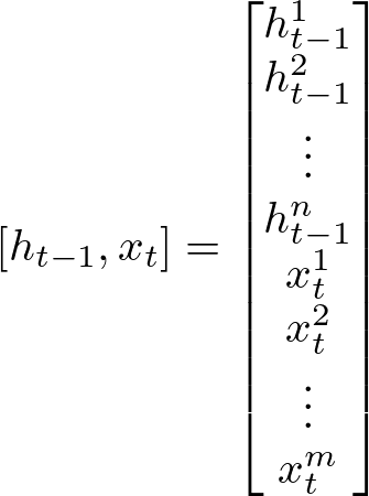
Let's focus for a moment on [_h t −1, _x t ], which represents the concatenation of the previous hidden state _h t −1 and the current input _x t . In the concatenation, two vectors are joined end-to-end to form a single larger vector. Suppose:
- _h t −1 is a vector of size n.
- _x t is a vector of size m.
Then the concatenated vector [_h t −1, _x t ] is a new vector of size n +m.
Mathematically, if:
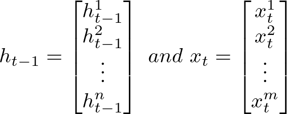 Previous hidden state vector (left) and current input x vector (right) - Image by Author
Then the concatenated vector [ht −1, xt ] is:
 Concatenated Vector - Image by Author
This new vector [_h t −1, _x t ] combines all the elements of _h t −1 followed by all the elements of _x t , forming a single column vector of size n +m. The concatenation ensures that both the past hidden state and the current input contribute to the calculation.
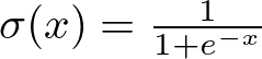
Let's now look at the role of the sigmoid function, σ , which is defined as:
 Sigmoid Function Formula - Image by Author
This function ensures that the values of the update gate _z t are between 0 and 1, which allows the gate to act as a filter. When _z t is close to 1, it means the GRU should retain a lot of the past information. When _z t is close to 0, it means the GRU should focus more on the new information.
Think of the update gate as a valve that controls the flow of information from the past to the present. If the valve is wide open (i.e., _z t is close to 1), a lot of the past information is allowed through. If the valve is nearly closed (i.e., _z t is close to 0), very little past information is carried forward.
This mechanism allows the GRU to strike a balance between remembering important past information and incorporating new data, which is crucial for tasks like language processing, where the context provided by previous words can be essential for understanding the current word.
3.2: Reset Gate
The reset gate in a GRU helps the model decide how much of the past information to forget. It's another crucial component that allows the GRU to manage dependencies over sequences effectively.
The reset gate _r t is calculated using the current input _x t and the previous hidden state _h t −1. The formula for the reset gate is:
 Reset Gate Formula - Image by Author
Here:
- _r_t _ is the reset gate at time step t.
- σ is the sigmoid activation function, which squashes the output between 0 and 1.
- _W_r _ is the weight matrix for the reset gate.
- _h t−1 is the hidden state from the previous time step.
- _x t is the current input.
- [_h t−1, _x t] is the concatenation of the previous hidden state and the current input, as described in the previous section.
Think of the reset gate as a switch that determines how much of the past should be ignored when considering new information. If the reset gate value _r t is close to 0, it means the past information should be largely forgotten. If _r t is close to 1, the past information is mostly retained.
In practical terms, the reset gate allows the GRU to selectively reset its memory, which can be particularly useful when the model needs to process a new sequence of data or when the context changes significantly.
3.3: Candidate Activation
The candidate activation in a GRU represents the new information that could potentially update the hidden state. This step integrates the reset gate's decision on how much past information to consider with the current input.
The candidate activation _h t is computed as follows:
 Candidate Activation Formula - Image by Author
Here:
- _h_t _ is the candidate activation at time step t.
- tanh is the hyperbolic tangent activation function, which outputs values between -1 and 1.
- W is the weight matrix for the candidate activation.
- _r t is the reset gate value at time step t (refer to section 3.2).
- _h t−1 is the hidden state from the previous time step.
- _x_t _ is the current input.
- [rt∗ ht−1,xt] represents the concatenation of the reset-modified previous hidden state and the current input.
In this case, we are replacing the sigmoid function with tanh. The tanh function is defined as:
 tanh Function Formula - Image by Author
This function outputs values between -1 and 1, allowing the GRU to introduce non-linearity into the model and control the range of the candidate activation.
Think of the candidate activation as a proposal for the new hidden state, combining the new input with the relevant past information. The reset gate _r t decides how much of the previous hidden state _h t −1 to include in this proposal.
If _r t is close to 0, the reset gate effectively zeros out the past hidden state, meaning the candidate activation relies heavily on the new input _x t . If _r t is close to 1, more of the past hidden state is considered, blending it with the new input to form _h t .
The candidate activation _h t then contributes to the final hidden state _h t for the current time step. The update gate _z t (refer to section 3.1) determines how much of this candidate activation is mixed with the previous hidden state:
 Updated Hidden State Formula - Image by Author
Where:
- _z t is the update gate value at time step t , calculated using the sigmoid function. It decides how much of the previous hidden state _h t −1 and the candidate activation _h t should contribute to the new hidden state.
- _h t−1 is the hidden state from the previous time step. It contains information about what the network has learned from the past inputs.
- _h t(tilde) is the candidate activation for the current time step, calculated using the reset gate and the current input. It represents the new information that could potentially update the hidden state.
- (1−_z t)∗_h t−1 controls how much of the previous hidden state is retained. When _z t is close to 0, the previous hidden state _h t −1 has a larger influence.
- _z t∗_h t (tilde) determines how much of the candidate activation _h t is added to the new hidden state. When _z t is close to 1, the candidate activation _h t has a larger influence.
By adjusting _z t , the GRU can smoothly transition between preserving past information and incorporating new information. This balance helps the GRU retain important historical context while adapting to new inputs, making it effective for handling sequential data with varying dependencies.
3.4: Step-by-Step Example
To understand how GRUs work in practice, let's walk through a simple example step-by-step. We'll use a small set of made-up numbers to illustrate the process.
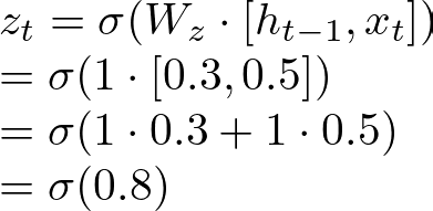
Let's assume:
- An input vector at time t , _x t = [0.5]
- A previous hidden state, _h t −1 = [0.3]
- Weights for the update gate, reset gate, and candidate activation are all 1 for simplicity.
- Biases are 0 for simplicity.
Step 1: Calculate the Update Gate First, we calculate the update gate _z t :
 Update Gate Calculation - Image by Author
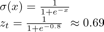
Using the sigmoid function:
 Sigmoid Function applied to Update Gate - Image by Author
Step 2: Calculate the Reset Gate Next, we calculate the reset gate _r t :
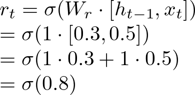 Reset Gate Calculation - Image by Author
Using the sigmoid function again:
 Sigmoid Function applied to Reset Gate - Image by Author
Step 3: Calculate the Candidate Activation Now, we calculate the candidate activation _h t :
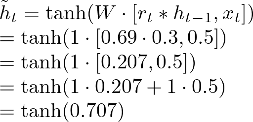 Candidate Activation Calculation - Image by Author
Using the tanh function:
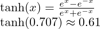 tanh Function applied to Candidate Activation - Image by Author
Step 4: Calculate the Final Hidden State Finally, we calculate the new hidden state _h t :
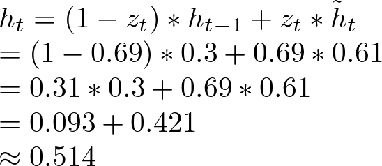 Final Hidden State Calculation - Image by Author
4: Building GRU From Scratch in Python
This section will guide you through implementing a Gated Recurrent Unit (GRU) network from scratch using Python. We will train the model over a flight passenger dataset. We will import the dataset from the seaborn library, which is free for commercial use.
You can find all the code we'll cover here:
models-from-scratch-python/Gated Recurrent Unit/demo.ipynb at main ·...
4.1: Imports and Custom Classes
First, we need to import the necessary libraries and custom classes that will help us build and train our GRU model. We'll use numpy for numerical operations, pandas for dataset manipulation, and seaborn for plotting. Additionally, we'll use custom classes for weight initialization and early stopping.
python
import numpy as np
import pandas as pd
import seaborn as sns

# Custom classes (built from scratch)
from src.model import WeightInitializer
from src.trainer import EarlyStopping
These custom classes (WeightInitializer and EarlyStopping) were created in a previous article. The WeightInitializer allows us to choose between several weight initialization techniques, and EarlyStopping stops the training process when there is no significant improvement in performance, preventing overfitting.
You can find the code for WeightInitializer and EarlyStopping in the article about LSTM:
The Math Behind LSTM
4.2: GRU Class
Here, we define the GRU class, which includes initialization, forward propagation, and backward propagation methods.
Initialization The __init__ method initializes the GRU with a specified input size , hidden size , and output size. It also initializes weights and biases using a custom weight initializer.
python
class GRU:
    def __init__(self, input_size, hidden_size, output_size, init_method='xavier'):
        self.input_size = input_size
        self.hidden_size = hidden_size
        self.output_size = output_size
        self.weight_initializer = WeightInitializer(method=init_method)

        # Initialize weights
        self.wz = self.weight_initializer.initialize((hidden_size, hidden_size + input_size))
        self.wr = self.weight_initializer.initialize((hidden_size, hidden_size + input_size))
        self.wh = self.weight_initializer.initialize((hidden_size, hidden_size + input_size))

        # Initialize biases
        self.bz = np.zeros((hidden_size, 1))
        self.br = np.zeros((hidden_size, 1))
        self.bh = np.zeros((hidden_size, 1))

        # Initialize output layer weights and biases
        self.why = self.weight_initializer.initialize((output_size, hidden_size))
        self.by = np.zeros((output_size, 1))
First, the initialization stores the sizes of the input, hidden, and output layers as class attributes. It also creates an instance of a WeightInitializer, using the specified method to initialize the weights, in this case, Xavier initialization.
Next, it initializes the weights for the update gate (wz), reset gate (wr), and candidate hidden state (wh). Each of these weights is a matrix that combines the hidden state and input dimensions.
After that, it initializes the biases for the update gate (bz), reset gate (br), and candidate hidden state (bh). These biases are vectors filled with zeros, one for each hidden unit.
Finally, it initializes the weights and biases for the output layer. The weights (why) are a matrix connecting the hidden state to the output, and the biases (by) are a vector filled with zeros, one for each output unit.
Activation Functions Next, we define static methods for the sigmoid function and its derivative, and the derivative of the tanh function.
less
    @staticmethod
    def sigmoid(z):
        return 1 / (1 + np.exp(-z))

    @staticmethod
    def dsigmoid(y):
        return y * (1 - y)

    @staticmethod
    def dtanh(y):
        return 1 - y * y
Forward Propagation The forward method processes the input through the GRU cell for each time step, calculating the reset and update gates, candidate activation, and the new hidden state.
python
    def forward(self, x):
        caches = []
        h_prev = np.zeros((self.hidden_size, 1))
        h = h_prev

        for t in range(x.shape[0]):
            x_t = x[t].reshape(-1, 1)
            combined = np.vstack((h_prev, x_t))

            z = self.sigmoid(np.dot(self.wz, combined) + self.bz)
            r = self.sigmoid(np.dot(self.wr, combined) + self.br)
            combined_r = np.vstack((r * h_prev, x_t))
            h_ = np.tanh(np.dot(self.wh, combined_r) + self.bh)

            h = (1 - z) * h_prev + z * h_

            cache = (h_prev, z, r, h_, x_t, combined, combined_r, h)
            caches.append(cache)

            h_prev = h

        y = np.dot(self.why, h) + self.by
        return y, caches
First, it initializes an empty list called caches to store intermediate values needed for backpropagation later. It also initializes the previous hidden state h_prev as a column vector of zeros with a size equal to the hidden layer size.
python
caches = []
h_prev = np.zeros((self.hidden_size, 1))
h = h_prev
Then, for each time step in the input sequence, it extracts the current input x_t and reshapes it into a column vector. It concatenates this input with the previous hidden state to form a combined input.
python
for t in range(x.shape[0]):
    x_t = x[t].reshape(-1, 1)
    combined = np.vstack((h_prev, x_t))
Next, it calculates the update gate z by applying the sigmoid function to the dot product of the update gate weights and the combined input, plus the update gate bias. Similarly, it calculates the reset gate r by applying the sigmoid function to the dot product of the reset gate weights and the combined input, plus the reset gate bias.
python
z = self.sigmoid(np.dot(self.wz, combined) + self.bz)
r = self.sigmoid(np.dot(self.wr, combined) + self.br)
The reset gate r is then used to modify the previous hidden state, which is concatenated with the current input to form combined_r. This combined input is then used to calculate the candidate hidden state h_ by applying the tanh function to the dot product of the candidate hidden state weights and combined_r, plus the candidate hidden state bias.
ini
combined_r = np.vstack((r * h_prev, x_t))
h_ = np.tanh(np.dot(self.wh, combined_r) + self.bh)
The new hidden state h is computed as a combination of the previous hidden state and the candidate hidden state, weighted by the update gate z.
ini
h = (1 - z) * h_prev + z * h_
All these intermediate values (h_prev, z, r, h_, x_t, combined, combined_r, and h) are stored in a tuple called cache, which is appended to the caches list.
cpp
cache = (h_prev, z, r, h_, x_t, combined, combined_r, h)
caches.append(cache)
The loop updates the previous hidden state h_prev to the current hidden state h for the next time step.
python
h_prev = h
After processing all time steps, the method calculates the final output y by applying the output layer weights and biases to the last hidden state.
python
y = np.dot(self.why, h) + self.by
Finally, the method returns the output y and the list of caches caches.
python
return y, caches
Backward Propagation The backward method calculates gradients using the caches from the forward pass and performs gradient clipping to prevent exploding gradients.
python
    def backward(self, dy, caches, clip_value=1.0):
        """
        Backward pass through the GRU network.

        Parameters:
        - dy: np.ndarray, gradient of the loss with respect to the output
        - caches: list, caches from the forward pass
        - clip_value: float, value to clip gradients to (default: 1.0)

        Returns:
        - tuple, gradients of the loss with respect to the parameters
        """
        # Initialize gradients
        dWz, dWr, dWh = [np.zeros_like(w) for w in (self.wz, self.wr, self.wh)]
        dbz, dbr, dbh = [np.zeros_like(b) for b in (self.bz, self.br, self.bh)]
        dWhy = np.zeros_like(self.why)
        dby = np.zeros_like(self.by)

        # Ensure dy is reshaped to match output size
        dy = dy.reshape(self.output_size, -1)
        dh_next = np.zeros((self.hidden_size, 1))  # shape must match hidden_size

        # Backpropagate through time
        for cache in reversed(caches):
            h_prev, z, r, h_, x_t, combined, combined_r, h = cache

            # Add gradient from next step to current output gradient
            dh = np.dot(self.why.T, dy) + dh_next
            dh_ = dh * z * self.dtanh(h_)
            dz = dh * (h_ - h_prev) * self.dsigmoid(z)
            dr = np.dot(self.wh[:, :self.hidden_size].T, dh_) * h_prev * self.dsigmoid(r)

            # Update gradients with respect to weights and biases
            dWz += np.dot(dz, combined.T)
            dWr += np.dot(dr, combined.T)
            dWh += np.dot(dh_, combined_r.T)

            dbz += dz.sum(axis=1, keepdims=True)
            dbr += dr.sum(axis=1, keepdims=True)
            dbh += dh_.sum(axis=1, keepdims=True)

            # Compute the gradient for the previous time step
            dh_prev = dh * (1 - z) + np.dot(self.wz[:, :self.hidden_size].T, dz) + np.dot(self.wr[:, :self.hidden_size].T, dr)

            dh_next = dh_prev

        # Update output layer weights and biases
        dWhy += np.dot(dy, h.T)
        dby += dy

        gradients = (dWz, dWr, dWh, dbz, dbr, dbh, dWhy, dby)

        # Gradient clipping
        for i in range(len(gradients)):
            np.clip(gradients[i], -clip_value, clip_value, out=gradients[i])

        return gradients
First, the method initializes gradients for the update gate weights (dWz), reset gate weights (dWr), candidate hidden state weights (dWh), and their respective biases (dbz, dbr, dbh). It also initializes gradients for the output layer weights (dWhy) and biases (dby). All these gradients are initialized to arrays of zeros with the same shape as the corresponding weights and biases.
python
dWz, dWr, dWh = [np.zeros_like(w) for w in (self.wz, self.wr, self.wh)]
dbz, dbr, dbh = [np.zeros_like(b) for b in (self.bz, self.br, self.bh)]
dWhy = np.zeros_like(self.why)
dby = np.zeros_like(self.by)
Next, the method reshapes the gradient of the loss with respect to the output (dy) to ensure it matches the output size. It also initializes dh_next, the gradient of the loss with respect to the next hidden state, to a column vector of zeros with a size equal to the hidden layer size.
python
dy = dy.reshape(self.output_size, -1)
dh_next = np.zeros((self.hidden_size, 1))
The method then iterates backward through the stored caches from the forward pass. For each cache, which contains intermediate values from a specific time step, it extracts the cached values: h_prev, z, r, h_, x_t, combined, combined_r, and h.
python
for cache in reversed(caches):
    h_prev, z, r, h_, x_t, combined, combined_r, h = cache
It calculates the gradient of the loss with respect to the hidden state (dh) by adding the gradient from the next time step (dh_next) to the dot product of the output layer weights transpose and dy. It then computes the gradients of the candidate hidden state (dh_), update gate (dz), and reset gate (dr).
python
# Add gradient from next step to current output gradient
dh = np.dot(self.why.T, dy) + dh_next
dh_ = dh * z * self.dtanh(h_)
dz = dh * (h_ - h_prev) * self.dsigmoid(z)
dr = np.dot(self.wh[:, :self.hidden_size].T, dh_) * h_prev * self.dsigmoid(r)
In this step, we update the gradients of the weights and biases. Specifically, it computes the gradients with respect to the combined input (dWz, dWr) and the combined reset input (dWh). It also updates the gradients of the biases (dbz, dbr, dbh).
python
# Update gradients with respect to weights and biases
dWz += np.dot(dz, combined.T)
dWr += np.dot(dr, combined.T)
dWh += np.dot(dh_, combined_r.T)

dbz += dz.sum(axis=1, keepdims=True)
dbr += dr.sum(axis=1, keepdims=True)
dbh += dh_.sum(axis=1, keepdims=True)
After that, it calculates the gradient of the loss with respect to the previous hidden state (dh_prev) to propagate the gradient back to the previous time step. The gradient dh_prev is a combination of the gradient of the loss with respect to the current hidden state and the contributions from the update gate and reset gate weights.
python
# Compute the gradient for the previous time step
dh_prev = dh * (1 - z) + np.dot(self.wz[:, :self.hidden_size].T, dz) + np.dot(self.wr[:, :self.hidden_size].T, dr)
This process continues for each time step, updating dh_next with dh_prev for the next iteration.
python
dh_next = dh_prev
Once the backpropagation through time is complete, the method updates the gradients of the output layer weights (dWhy) and biases (dby) using the gradient of the loss with respect to the output.
python
# Update output layer weights and biases
dWhy += np.dot(dy, h.T)
dby += dy
Finally, it clips the gradients to a specified value (clip_value) to prevent exploding gradients, ensuring that all gradient values are within the range [-clip_value, clip_value]. The method returns the computed gradients for all parameters as a tuple.
python
gradients = (dWz, dWr, dWh, dbz, dbr, dbh, dWhy, dby)

# Gradient clipping
for i in range(len(gradients)):
    np.clip(gradients[i], -clip_value, clip_value, out=gradients[i])

return gradients
Updating Parameters The update_params method applies the gradients to update the model parameters.
python
    def update_params(self, grads, learning_rate):
        dWz, dWr, dWh, dbz, dbr, dbh, dWhy, dby = grads

        self.wz -= learning_rate * dWz
        self.wr -= learning_rate * dWr
        self.wh -= learning_rate * dWh

        self.bz -= learning_rate * dbz
        self.br -= learning_rate * dbr
        self.bh -= learning_rate * dbh

        self.why -= learning_rate * dWhy
        self.by -= learning_rate * dby
First, the method unpacks the grads tuple into individual gradient variables: dWz, dWr, dWh, dbz, dbr, dbh, dWhy, and dby. These represent the gradients of the loss with respect to the update gate weights, reset gate weights, candidate hidden state weights, their corresponding biases, and the output layer weights and biases, respectively.
Then, for each parameter, the method performs a gradient descent step. Specifically, it subtracts the product of the gradient and the learning rate from the current value of the parameter. This operation is performed for the update gate weights (wz), reset gate weights (wr), candidate hidden state weights (wh), their biases (bz, br, bh), and the output layer weights (why) and biases (by).
Therefore, this method adjusts the parameters of the GRU network in the direction that reduces the loss. The learning rate controls how big each adjustment step is, ensuring that the parameters are updated incrementally based on the gradients calculated during backpropagation. This process is repeated for each parameter, resulting in an updated set of weights and biases for the network.
4.3: GRUTrainer Class
The GRUTrainer class handles the training process, including forward and backward passes, and updates the model parameters.
Initialization The __init__ method initializes the trainer with the GRU model, learning rate, and early stopping criteria.
python
class GRUTrainer:
    def __init__(self, model, learning_rate=0.01, patience=7, verbose=True, delta=0):
        self.model = model
        self.learning_rate = learning_rate
        self.train_losses = []
        self.val_losses = []
        self.early_stopping = EarlyStopping(patience, verbose, delta)
This class takes four parameters: model, which is the GRU model to be trained; learning_rate, which specifies the step size for updating the model's parameters during training (default is 0.01); patience, which defines how many epochs to wait for an improvement in validation loss before stopping the training early (default is 7); and verbose, a boolean that controls whether to print training information (default is True). It also accepts delta, which is the minimum change in validation loss to qualify as an improvement (default is 0).
Inside the __init__ method, it sets these parameters as attributes of the GRUTrainer instance. It initializes an empty list train_losses to keep track of the training loss for each epoch and another empty list val_losses to store the validation loss for each epoch.
Finally, it initializes an instance of EarlyStopping with the given patience, verbose, and delta parameters. This instance will be used to monitor the validation loss and determine when to stop training if the loss does not improve within the specified patience period.
Training Method The train method trains the GRU model on the training data and optionally validates it on a separate validation set.
python
    def train(self, X_train, y_train, X_val=None, y_val=None, epochs=10, batch_size=1, clip_value=1.0):
        for epoch in range(epochs):
            epoch_losses = []
            for i in range(0, len(X_train), batch_size):
                batch_X = X_train[i:i + batch_size]
                batch_y = y_train[i:i + batch_size]
                losses = []

                for x, y_true in zip(batch_X, batch_y):
                    y_pred, caches = self.model.forward(x)
                    loss = self.compute_loss(y_pred, y_true.reshape(-1, 1))
                    losses.append(loss)

                    dy = y_pred - y_true.reshape(-1, 1)
                    grads = self.model.backward(dy, caches, clip_value=clip_value)
                    self.model.update_params(grads, self.learning_rate)

                batch_loss = np.mean(losses)
                epoch_losses.append(batch_loss)

            avg_epoch_loss = np.mean(epoch_losses)
            self.train_losses.append(avg_epoch_loss)

            if X_val is not None and y_val is not None:
                val_loss = self.validate(X_val, y_val)
                self.val_losses.append(val_loss)

                if epoch % 10 == 0:
                    print(f'Epoch {epoch + 1}/{epochs} - Loss: {avg_epoch_loss:.5f}, Val Loss: {val_loss:.5f}')

                self.early_stopping(val_loss)
                if self.early_stopping.early_stop:
                    print("Early stopping")
                    break
            else:
                print(f'Epoch {epoch + 1}/{epochs} - Loss: {avg_epoch_loss:.5f}')
First, the method iterates through the number of epochs specified. For each epoch, it initializes an empty list epoch_losses to store the loss for each batch.
python
for epoch in range(epochs):
    epoch_losses = []
Within each epoch, it iterates over the training data in mini-batches of size batch_size. For each batch, it extracts the current batch of inputs (batch_X) and their corresponding labels (batch_y). It initializes an empty list losses to store the loss for each sample in the batch.
python
for i in range(0, len(X_train), batch_size):
    batch_X = X_train[i:i + batch_size]
    batch_y = y_train[i:i + batch_size]
    losses = []
For each sample in the current batch, it performs the forward pass by calling the forward method of the GRU model, which returns the predicted output (y_pred) and the caches containing intermediate values needed for backpropagation. It then computes the loss between the predicted output and the true label (y_true), reshaped to match the prediction's shape, and appends this loss to the losses list.
python
for x, y_true in zip(batch_X, batch_y):
    y_pred, caches = self.model.forward(x)
    loss = self.compute_loss(y_pred, y_true.reshape(-1, 1))
    losses.append(loss)
Next, it computes the gradient of the loss with respect to the output (dy) and performs backpropagation by calling the backward method of the GRU model, which returns the gradients for the model's parameters. It then updates the model's parameters using these gradients by calling the update_params method with the computed gradients and the learning rate.
python
dy = y_pred - y_true.reshape(-1, 1)
grads = self.model.backward(dy, caches, clip_value=clip_value)
self.model.update_params(grads, self.learning_rate)
After processing all samples in the current batch, it calculates the mean loss for the batch (batch_loss) and appends it to the epoch_losses list.
go
batch_loss = np.mean(losses)
epoch_losses.append(batch_loss)
Once all batches are processed for the current epoch, it calculates the average loss for the epoch (avg_epoch_loss) and appends it to the train_losses list.
python
avg_epoch_loss = np.mean(epoch_losses)
self.train_losses.append(avg_epoch_loss)
If validation data is provided (X_val, y_val), the method validates the model by calling the validate method, which returns the validation loss (val_loss). This validation loss is appended to the val_losses list.
python
if X_val is not None and y_val is not None:
    val_loss = self.validate(X_val, y_val)
    self.val_losses.append(val_loss)
Every 10 epochs, the method prints the current epoch number, the average training loss, and the validation loss if available.
python
if epoch % 10 == 0:
    print(f'Epoch {epoch + 1}/{epochs} - Loss: {avg_epoch_loss:.5f}, Val Loss: {val_loss:.5f}')

    self.early_stopping(val_loss)
The method then checks for early stopping by calling the early_stopping method with the current validation loss. If early stopping is triggered, indicated by the early_stop attribute of early_stopping being True, it prints a message and breaks out of the training loop.
lua
if self.early_stopping.early_stop:
    print("Early stopping")
    break
If validation data is not provided, it simply prints the current epoch number and the average training loss for each epoch.
python
else:
    print(f'Epoch {epoch + 1}/{epochs} - Loss: {avg_epoch_loss:.5f}')
Compute Loss and Validate Methods The compute_loss method calculates the mean squared error loss and the validate method evaluates the model on validation data.
python
def compute_loss(self, y_pred, y_true):
    return np.mean((y_pred - y_true) ** 2)
The compute_loss method in the GRUTrainer class calculates the mean squared error loss between the predicted output (y_pred) and the true label (y_true). This method takes two arguments: y_pred, the predictions made by the model, and y_true, the actual labels. It computes the element-wise difference between y_pred and y_true, squares these differences, and then takes the mean of these squared differences to get the mean squared error loss.
python
def validate(self, X_val, y_val):
    val_losses = []
    for x, y_true in zip(X_val, y_val):
        y_pred, _ = self.model.forward(x)
        loss = self.compute_loss(y_pred, y_true.reshape(-1, 1))
        val_losses.append(loss)
    return np.mean(val_losses)
The validate method evaluates the model on a separate validation dataset to check its performance. This method takes two arguments: X_val, the validation inputs, and y_val, the validation labels.
First, it initializes an empty list val_losses to store the loss for each validation sample. It then iterates over each sample in the validation dataset, extracting the input x and the corresponding true label y_true.
For each sample, it performs the forward pass by calling the forward method of the GRU model, which returns the predicted output (y_pred). It then computes the loss between the predicted output and the true label, reshaped to match the prediction's shape, by calling the compute_loss method. This loss is appended to the val_losses list.
After processing all validation samples, it calculates the mean of the collected losses (val_losses) and returns this mean value as the validation loss. This provides an overall measure of the model's performance on the validation dataset.
4.4: TimeSeriesDataset Class
The TimeSeriesDataset class is designed to handle time series data, specifically for loading, preprocessing, and creating datasets suitable for training and testing a model. It takes two optional parameters: look_back, which determines the number of previous time steps to use as input features (default is 1), and train_size, which specifies the proportion of data to be used for training (default is 0.67).
python
class TimeSeriesDataset:
    def __init__(self, look_back=1, train_size=0.67):
        self.look_back = look_back
        self.train_size = train_size

    def load_data(self):
        df = sns.load_dataset('flights')
        df['Date']  = pd.to_datetime(df['year'].astype(str) + '-' + df['month'].astype(str) + '-01')
        df = df.set_index('Date')
        df = df.drop(['year', 'month'], axis=1)
        df = df.values.astype(float)
        df = self.MinMaxScaler(df)
        train_size = int(len(df) * self.train_size)
        train, test = df[0:train_size,:], df[train_size:len(df),:]
        return train, test

    def MinMaxScaler(self, data):
        numerator = data - np.min(data, 0)
        denominator = np.max(data, 0) - np.min(data, 0)
        return numerator / (denominator + 1e-7)

    def create_dataset(self, dataset):
        dataX, dataY = []
        for i in range(len(dataset)-self.look_back):
            a = dataset[i:(i + self.look_back), 0]
            dataX.append(a)
            dataY.append(dataset[i + self.look_back, 0])
        return np.array(dataX), np.array(dataY)

    def get_train_test(self):
        train, test = self.load_data()
        trainX, trainY = self.create_dataset(train)
        testX, testY = self.create_dataset(test)
        return trainX, trainY, testX, testY
The load_data method loads a dataset of flight data using Seaborn's load_dataset function. It converts the 'year' and 'month' columns into a datetime format and sets this datetime as the index, it then drops the original 'year' and 'month' columns, leaving only the 'passengers' column. The method converts this column to a float type and scales the values between 0 and 1 using the MinMaxScaler method. It then splits the scaled data into training and testing sets based on the train_size attribute. The training set consists of the first train_size proportion of the data, and the testing set consists of the remaining data. The method returns these two sets.
python
def load_data(self):
    df = sns.load_dataset('flights')
    df['Date']  = pd.to_datetime(df['year'].astype(str) + '-' + df['month'].astype(str) + '-01')
    df = df.set_index('Date')
    df = df.drop(['year', 'month'], axis=1)
    df = df.values.astype(float)
    df = self.MinMaxScaler(df)
    train_size = int(len(df) * self.train_size)
    train, test = df[0:train_size,:], df[train_size:len(df),:]
    return train, test
The MinMaxScaler method takes in the data and normalizes it. It subtracts the minimum value of each feature from the data and then divides it by the range (maximum value minus minimum value) of each feature. This ensures that the data values are scaled between 0 and 1.
python
def MinMaxScaler(self, data):
    numerator = data - np.min(data, 0)
    denominator = np.max(data, 0) - np.min(data, 0)
    return numerator / (denominator + 1e-7)
The create_dataset method creates input-output pairs for the model. It takes the dataset and initializes two empty lists, dataX and dataY. For each time step in the dataset (up to len(dataset) - self.look_back), it creates a sequence of self.look_back previous time steps as the input (dataX) and the next time step as the output (dataY). These pairs are appended to the respective lists. The method returns these lists as numpy arrays.
python
def create_dataset(self, dataset):
    dataX, dataY = []
    for i in range(len(dataset)-self.look_back):
        a = dataset[i:(i + self.look_back), 0]
        dataX.append(a)
        dataY.append(dataset[i + self.look_back, 0])
    return np.array(dataX), np.array(dataY)
The get_train_test method combines the previous methods to produce the final training and testing datasets. It first calls load_data to obtain the training and testing sets. Then, it calls create_dataset on each set to generate the input-output pairs for both training and testing. Finally, it returns the training inputs (trainX), training outputs (trainY), testing inputs (testX), and testing outputs (testY). This method provides a complete pipeline for preparing the data for training and testing a model.
python
def get_train_test(self):
    train, test = self.load_data()
    trainX, trainY = self.create_dataset(train)
    testX, testY = self.create_dataset(test)
    return trainX, trainY, testX, testY
4.5: Training the GRU Model
First, we instantiate the TimeSeriesDataset class with a train_size of 0.7, meaning 70% of the data will be used for training and a look_back of 1, meaning each input feature will consist of one previous time step. We call the get_train_test method of the dataset instance to obtain the training and testing datasets. The method returns four arrays: trainX, trainY, testX, and testY.
python
# Instantiate the dataset
dataset = TimeSeriesDataset(train_size=0.7, look_back=1)
trainX, trainY, testX, testY = dataset.get_train_test()
Next, we reshape trainX and testX to be in the format [samples, time steps, features]. This is done using NumPy's reshape function. For trainX, the new shape is (number of samples, number of time steps, 1), where the last dimension represents the single feature (passenger count). The same reshaping is applied to testX.
python
# Reshape input to be [samples, time steps, features]
trainX = np.reshape(trainX, (trainX.shape[0], trainX.shape[1], 1))
testX = np.reshape(testX, (testX.shape[0], testX.shape[1], 1))
We then instantiate the GRU class with an input_size of 1 (since each input has one feature), a hidden_size of 256 (the number of GRU units in the hidden layer), and an output_size of 1 (since we want to predict one value, the passenger count for the next time step).
python
gru = GRU(input_size=1, hidden_size=256, output_size=1)
Next, we instantiate the GRUTrainer class, passing in the GRU model instance. We set the learning_rate to 0.001, patience to 50 (the number of epochs to wait for an improvement in validation loss before stopping early), verbose to True (so training information will be printed), and delta to 0.001 (the minimum change in validation loss to qualify as an improvement).
python
trainer = GRUTrainer(gru, learning_rate=1e-3, patience=50, verbose=True, delta=0.001)
Finally, we call the train method of the GRUTrainer instance to train the GRU model. We pass in the reshaped training and testing datasets (trainX, trainY, testX, testY), set the number of training epochs to 1000, the batch size to 32, and the gradient clipping value to 1.0. The training process will iteratively update the model's parameters to minimize the loss of the training data while monitoring the validation loss for early stopping.
python
trainer.train(trainX, trainY, testX, testY, epochs=1000, batch_size=32)
5: Conclusion
In this article, we explored Gated Recurrent Units (GRUs) and how they work. We started by comparing GRUs to LSTMs and Vanilla RNNs, then broke down the math behind key components like the update gate, reset gate, and candidate activation. We also provided a step-by-step guide to implementing a GRU from scratch in Python, with clear explanations of the code. Understanding and building GRUs helps us handle sequential data effectively, making them useful for tasks like time series prediction and natural language processing.
References
- Cho, Kyunghyun, et al. "Learning phrase representations using RNN encoder-decoder for statistical machine translation." arXiv preprint arXiv:1406.1078 (2014).
- Towards Data Science. "The Math Behind Recurrent Neural Networks." Towards Data Science (2020). Link to Article
- Towards Data Science. "The Math Behind LSTM." Towards Data Science (2020). Link to Article
Register Now to Continue Reading
Unlock Towards Data Science with a Free Account
All articles on Towards Data Science are available to registered users. Create a free account today to access this article and thousands more.
Register for freeSign in to your account
 Written By
See all from Cristian Leo
Deep DivesDeep LearningMachine LearningMathematicsPython
Share This Article
Towards Data Science is a community publication. Submit your insights to reach our global audience and earn through the TDS Author Payment Program.
Write for TDS
Related Articles
Data Engineering
A small experiment in remote SQL execution
Thomas Reid
August 16, 202617 min read
Programming
Let's dig in to the more formal details of OOP.
Mark Douthwaite
October 9, 202012 min read
Machine Learning
An Introductory Guide and Use Case for Applied Data Science
Kurt Klingensmith
August 8, 202413 min read
Machine Learning
ML Maturity in Industry
Tom Martin
May 3, 202210 min read
Deep Learning
How I built a real-time, standalone traffic monitoring and analytics system
J. Rafid Siddiqui, PhD
March 6, 20227 min read
Artificial Intelligence
Neural Networks are the programmable patterns that helps to solve complex problems and bring the best achievable output. Deep Learning as...
Aarya Brahmane
October 26, 202010 min read
Machine Learning
Improve Your Workflows and Productivity With Wolfram
Arnoud Buzing
September 21, 20203 min read
Programming
Leverage SQL indexing to speed up your queries. Learn when to index, when not to, and how indexing works under the hood.
Christopher Karg
November 8, 202419 min read
Large Language Model
Enterprise Document Intelligence [Vol.1 #13] - Putting the patterns together, and why this is what “agentic RAG” should look like
Angela and Kezhan Shi
August 14, 202627 min read
Your home for data science and AI. The world's leading publication for data science, data analytics, data engineering, machine learning, and artificial intelligence professionals.
Subscribe to Our NewsletterWrite For TDS•About•Advertise•Privacy Policy•Terms of Use
© Insight Media Group, LLC 2026•The New Stack•roadmap.sh•Creator Network
Recommended Articles
Close