保留正文与补采附件。源页面当前未重新核验;具体限制见交付清单。
 We value your privacy
We use cookies to enhance your browsing experience, serve personalised ads or content, and analyse our traffic. By clicking "Accept All", you consent to our use of cookies.
Customise Reject All Accept All
Customise Consent Preferences
 We use cookies to help you navigate efficiently and perform certain functions. You will find detailed information about all cookies under each consent category below.
The cookies that are categorised as "Necessary" are stored on your browser as they are essential for enabling the basic functionalities of the site. ... Show more
NecessaryAlways Active
Necessary cookies are required to enable the basic features of this site, such as providing secure log-in or adjusting your consent preferences. These cookies do not store any personally identifiable data.
-
Cookie
BCTempID
-
Duration
10 minutes
-
Description
No description available.
-
Cookie
__cf_bm
-
Duration
1 hour
-
Description
This cookie, set by Cloudflare, is used to support Cloudflare Bot Management.
-
Cookie
AWSALBCORS
-
Duration
7 days
-
Description
Amazon Web Services set this cookie for load balancing.
-
Cookie
_cfuvid
-
Duration
session
-
Description
Cloudflare sets this cookie to track users across sessions to optimize user experience by maintaining session consistency and providing personalized services
-
Cookie
li_gc
-
Duration
6 months
-
Description
Linkedin set this cookie for storing visitor's consent regarding using cookies for non-essential purposes.
-
Cookie
__hssrc
-
Duration
session
-
Description
This cookie is set by Hubspot whenever it changes the session cookie. The __hssrc cookie set to 1 indicates that the user has restarted the browser, and if the cookie does not exist, it is assumed to be a new session.
-
Cookie
__hssc
-
Duration
1 hour
-
Description
HubSpot sets this cookie to keep track of sessions and to determine if HubSpot should increment the session number and timestamps in the __hstc cookie.
-
Cookie
wpEmojiSettingsSupports
-
Duration
session
-
Description
WordPress sets this cookie when a user interacts with emojis on a WordPress site. It helps determine if the user's browser can display emojis properly.
-
Cookie
BCSessionID
-
Duration
1 year 1 month 4 days
-
Description
Blueconic sets this cookie as a unique identifier for the BlueConic profile.
-
Cookie
_octo
-
Duration
1 year
-
Description
No description available.
-
Cookie
logged_in
-
Duration
1 year
-
Description
No description available.
-
Cookie
__Secure-YEC
-
Duration
past
-
Description
YouTube sets this cookie to stores the user's video player preferences using embedded YouTube video
-
Cookie
__eoi
-
Duration
6 months
-
Description
Description is currently not available.
-
Cookie
AWSALBTGCORS
-
Duration
7 days
-
Description
No description available.
-
Cookie
login-status-p
-
Duration
past
-
Description
Description is currently not available.
-
Cookie
AWSALBTG
-
Duration
7 days
-
Description
No description available.
-
Cookie
csrf_token
-
Duration
session
-
Description
No description available.
-
Cookie
token_v2
-
Duration
1 day
-
Description
Description is currently not available.
-
Cookie
D
-
Duration
1 year
-
Description
Description is currently not available.
-
Cookie
PHPSESSID
-
Duration
session
-
Description
This cookie is native to PHP applications. The cookie stores and identifies a user's unique session ID to manage user sessions on the website. The cookie is a session cookie and will be deleted when all the browser windows are closed.
-
Cookie
VISITOR_PRIVACY_METADATA
-
Duration
6 months
-
Description
YouTube sets this cookie to store the user's cookie consent state for the current domain.
-
Cookie
cookietest
-
Duration
session
-
Description
The cookietest cookie is typically used to determine whether the user's browser accepts cookies, essential for website functionality and user experience.
-
Cookie
__Host-airtable-session
-
Duration
1 year
-
Description
This cookie is used to enable us to integrate the services of Airtable.
-
Cookie
__Host-airtable-session.sig
-
Duration
1 year
-
Description
This cookie is used to enable us to integrate the services of Airtable.
-
Cookie
m
-
Duration
1 year 1 month 4 days
-
Description
Stripe sets this cookie for fraud prevention purposes. It identifies the device used to access the website, allowing the website to be formatted accordingly.
-
Cookie
BIGipServer*
-
Duration
session
-
Description
Marketo sets this cookie to collect information about the user's online activity and build a profile about their interests to provide advertisements relevant to the user.
-
Cookie
__cfruid
-
Duration
session
-
Description
Cloudflare sets this cookie to identify trusted web traffic.
-
Cookie
_GRECAPTCHA
-
Duration
6 months
-
Description
Google Recaptcha service sets this cookie to identify bots to protect the website against malicious spam attacks.
-
Cookie
__Secure-YNID
-
Duration
6 months
-
Description
Google cookie used to protect user security and prevent fraud, especially during the login process.
-
Cookie
cookieyes-consent
-
Duration
1 year
-
Description
CookieYes sets this cookie to remember users' consent preferences so that their preferences are respected on subsequent visits to this site. It does not collect or store any personal information about the site visitors.
Functional
Functional cookies help perform certain functionalities like sharing the content of the website on social media platforms, collecting feedback, and other third-party features.
-
Cookie
lidc
-
Duration
1 day
-
Description
LinkedIn sets the lidc cookie to facilitate data center selection.
-
Cookie
brw
-
Duration
1 year
-
Description
No description available.
-
Cookie
brwConsent
-
Duration
5 minutes
-
Description
Description is currently not available.
-
Cookie
WMF-Uniq
-
Duration
1 year
-
Description
Description is currently not available.
-
Cookie
loom_anon_comment
-
Duration
1 year
-
Description
No description available.
-
Cookie
loom_referral_video
-
Duration
session
-
Description
Description is currently not available.
-
Cookie
VISITOR_INFO1_LIVE
-
Duration
6 months
-
Description
A cookie set by YouTube to measure bandwidth that determines whether the user gets the new or old player interface.
-
Cookie
yt-remote-connected-devices
-
Duration
Never Expires
-
Description
YouTube sets this cookie to store the user's video preferences using embedded YouTube videos.
-
Cookie
ytidb::LAST_RESULT_ENTRY_KEY
-
Duration
Never Expires
-
Description
The cookie ytidb::LAST_RESULT_ENTRY_KEY is used by YouTube to store the last search result entry that was clicked by the user. This information is used to improve the user experience by providing more relevant search results in the future.
-
Cookie
yt-remote-device-id
-
Duration
Never Expires
-
Description
YouTube sets this cookie to store the user's video preferences using embedded YouTube videos.
-
Cookie
yt-remote-session-name
-
Duration
session
-
Description
The yt-remote-session-name cookie is used by YouTube to store the user's video player preferences using embedded YouTube video.
-
Cookie
yt-remote-fast-check-period
-
Duration
session
-
Description
The yt-remote-fast-check-period cookie is used by YouTube to store the user's video player preferences for embedded YouTube videos.
-
Cookie
yt-remote-session-app
-
Duration
session
-
Description
The yt-remote-session-app cookie is used by YouTube to store user preferences and information about the interface of the embedded YouTube video player.
-
Cookie
yt-remote-cast-available
-
Duration
session
-
Description
The yt-remote-cast-available cookie is used to store the user's preferences regarding whether casting is available on their YouTube video player.
-
Cookie
yt-remote-cast-installed
-
Duration
session
-
Description
The yt-remote-cast-installed cookie is used to store the user's video player preferences using embedded YouTube video.
-
Cookie
cp_session
-
Duration
3 months
-
Description
Codepen sets this cookie for Help systems found in the website.
-
Cookie
loid
-
Duration
1 year 1 month 4 days
-
Description
This cookie is set by the Reddit. The cookie enables the sharing of content from the website onto the social media platform.
Analytics
Analytical cookies are used to understand how visitors interact with the website. These cookies help provide information on metrics such as the number of visitors, bounce rate, traffic source, etc.
-
Cookie
__hstc
-
Duration
6 months
-
Description
Hubspot set this main cookie for tracking visitors. It contains the domain, initial timestamp (first visit), last timestamp (last visit), current timestamp (this visit), and session number (increments for each subsequent session).
-
Cookie
hubspotutk
-
Duration
6 months
-
Description
HubSpot sets this cookie to keep track of the visitors to the website. This cookie is passed to HubSpot on form submission and used when deduplicating contacts.
-
Cookie
_ga
-
Duration
1 year 1 month 4 days
-
Description
Google Analytics sets this cookie to calculate visitor, session and campaign data and track site usage for the site's analytics report. The cookie stores information anonymously and assigns a randomly generated number to recognise unique visitors.
-
Cookie
ga*
-
Duration
1 year 1 month 4 days
-
Description
Google Analytics sets this cookie to store and count page views.
-
Cookie
__Host-psifi.analyticsTrace
-
Duration
6 hours
-
Description
Description is currently not available.
-
Cookie
__Host-psifi.analyticsTraceV2
-
Duration
6 hours
-
Description
Description is currently not available.
-
Cookie
_gh_sess
-
Duration
session
-
Description
GitHub sets this cookie for temporary application and framework state between pages like what step the user is on in a multiple step form.
-
Cookie
YSC
-
Duration
session
-
Description
YSC cookie is set by Youtube and is used to track the views of embedded videos on Youtube pages.
-
Cookie
ajs_anonymous_id
-
Duration
1 year
-
Description
This cookie is set by Segment to count the number of people who visit a certain site by tracking if they have visited before.
-
Cookie
vuid
-
Duration
1 year 1 month 4 days
-
Description
Vimeo installs this cookie to collect tracking information by setting a unique ID to embed videos on the website.
Performance
Performance cookies are used to understand and analyse the key performance indexes of the website which helps in delivering a better user experience for the visitors.
-
Cookie
AWSALB
-
Duration
7 days
-
Description
AWSALB is an application load balancer cookie set by Amazon Web Services to map the session to the target.
-
Cookie
acq
-
Duration
past
-
Description
Description is currently not available.
-
Cookie
acq.sig
-
Duration
past
-
Description
Description is currently not available.
-
Cookie
ptc
-
Duration
2 years
-
Description
No description available.
Advertisement
Advertisement cookies are used to provide visitors with customised advertisements based on the pages you visited previously and to analyse the effectiveness of the ad campaigns.
-
Cookie
muc_ads
-
Duration
1 year 1 month 4 days
-
Description
Twitter sets this cookie to collect user behaviour and interaction data to optimize the website.
-
Cookie
guest_id_marketing
-
Duration
1 year 1 month 4 days
-
Description
Twitter sets this cookie to identify and track the website visitor.
-
Cookie
guest_id_ads
-
Duration
1 year 1 month 4 days
-
Description
Twitter sets this cookie to identify and track the website visitor.
-
Cookie
personalization_id
-
Duration
1 year 1 month 4 days
-
Description
Twitter sets this cookie to integrate and share features for social media and also store information about how the user uses the website, for tracking and targeting.
-
Cookie
guest_id
-
Duration
1 year 1 month 4 days
-
Description
Twitter sets this cookie to identify and track the website visitor. It registers if a user is signed in to the Twitter platform and collects information about ad preferences.
-
Cookie
bcookie
-
Duration
1 year
-
Description
LinkedIn sets this cookie from LinkedIn share buttons and ad tags to recognize browser IDs.
-
Cookie
__Secure-ROLLOUT_TOKEN
-
Duration
6 months
-
Description
YouTube sets this cookie to manage feature rollout and experimentation. It helps Google control which new features or interface changes are shown to users as part of testing and staged rollouts, ensuring consistent experience for a given user during an experiment.
-
Cookie
yt.innertube::nextId
-
Duration
Never Expires
-
Description
YouTube sets this cookie to register a unique ID to store data on what videos from YouTube the user has seen.
-
Cookie
yt.innertube::requests
-
Duration
Never Expires
-
Description
YouTube sets this cookie to register a unique ID to store data on what videos from YouTube the user has seen.
-
Cookie
session_tracker
-
Duration
session
-
Description
This cookie is set by the Reddit. This cookie is used to identify trusted web traffic. It also helps in adverstising on the website.
-
Cookie
edgebucket
-
Duration
session
-
Description
Reddit sets this cookie to save the information about a log-on Reddit user, for the purpose of advertisement recommendations and updating the content.
-
Cookie
did
-
Duration
1 year
-
Description
Arbor sets this cookie to show targeted ads to site visitors.This cookie expires after 2 months or 1 year.
Uncategorised
Other uncategorised cookies are those that are being analysed and have not been classified into a category as yet.
No cookies to display.
Reject All Save My Preferences Accept All
Toggle SearchToggle Mobile Navigation
Publish AI, ML & data-science insights to a global community of data professionals.
Sign inSubmit an Article
LatestEditor's PicksNewsletterShipAI
Write For TDS
LinkedInXToggle Search
Machine Learning
Classifying Handwritten Digits Using A Multilayer Perceptron Classifier (MLP)
What is a Multilayer Perceptron? What are the pros and cons of MLP? Can we classify handwritten digits accurately using a MLP classifier...
Serafeim Loukas, PhD
November 27, 20217 min read
What is a Multilayer Perceptron? What are the pros and cons of MLP? Can we classify handwritten digits accurately using a MLP classifier? How do learnt weights look like?
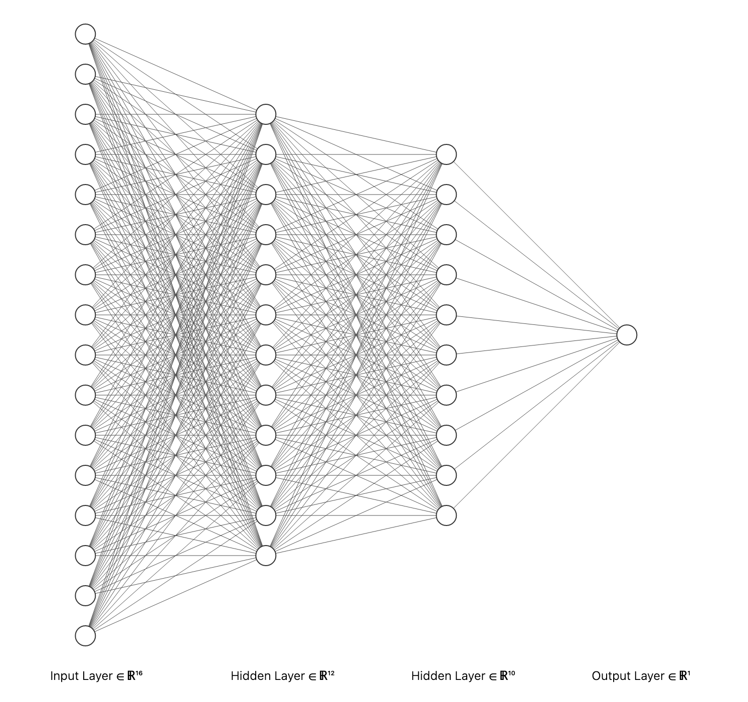 Figure 1: A Multilayer Perceptron Network (source).
Learn this step by step with the interactive Machine Learning roadmap.
1. Short Introduction
1.1 What is a Multilayer Perceptron (MLP)?
An MLP is a supervised machine learning (ML) algorithm that belongs in the class of feedforward artificial neural networks [1]. The algorithm essentially is trained on the data in order to learn a function. Given a set of features and a target variable (e.g. labels) it learns a non-linear function for either classification or regression. In this article, we will only focus on the classification case.
1.2 Is there any similarity between the MLP and the Logistic Regression?
There is! The logistic regression has only two layers i.e. the input and output however, in the case of a MLP model, the only difference is that we can have additional intermediate nonlinear layers. These are known as hidden layers. Except for the input nodes (nodes that belong to the input layer), each node is a neuron that uses a nonlinear activation function [1]. Due to this non-linearity nature, the MLP can learn complex nonlinear functions and thus, distinguish data that are not linearly separable! See Figure 2 below for a visual representation of an MLP classifier with one hidden layer.
NEW : After a great deal of hard work and staying behind the scenes for quite a while, we're excited to now offer our expertise through a platform, the "Data Science Hub" on Patreon (https://www.patreon.com/TheDataScienceHub). This hub is our way of providing you with bespoke consulting services and comprehensive responses to all your inquiries , ranging from Machine Learning to strategic data analytics planning.
1.3 How is an MLP trained?
MLP uses backpropagation for training [1]. You can have a look at this website here for the formal mathematical formulation.
1.4 Main Advantages and Disadvantages of MLP
Pros
- Can learn nonlinear functions and thus separate not linearly separable data [2].
Cons
- The loss function for the hidden layer leads to a non -convex optimization problem and thus, local minimum exist.
- Due to the above issue, different weight initializations may lead to different outputs/weights/results.
- The MLP has some hyperparameters e.g. the number of hidden neurons, layers that need to be tuned (time & power consuming) [2].
- MLP can be sensitive to feature scaling [2].
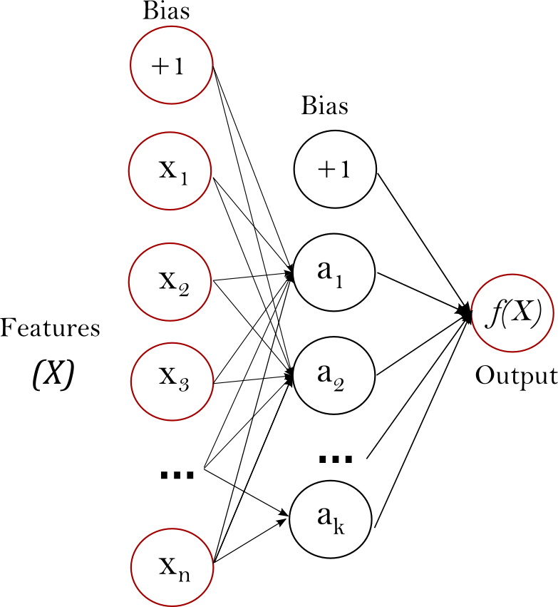 Figure 2: A MLP with one hidden layer and with a scalar output. Image adapted from scikit-learn python documentation.
2. Python hands-on example using scikit-learn
2.1 The dataset
For this hands-on example we will use the MNIST dataset. The MNIST database is famous database of handwritten digits that is used for training several ML models [5]. There are handwritten images of 10 different digits so the number of classes is **10**(see Figure 3).
Note : Since we deal with images , these are represented by 2D arrays and the initial dimension of the data is 28** by **28 for each image (28x28 pixels). The 2D images are then flattened and thus, represented by vectors at the end. Each 2D image is transformed into a 1D vector with dimension [1, 28x28] = **[1, 784]. Finally, our dataset has _784 features/variables/columns.**_
 Figure 3: Some samples from the dataset (Source).
2.2 Data import and preparation
text
import matplotlib.pyplot as plt
from sklearn.datasets import fetch_openml
from sklearn.neural_network import MLPClassifier

# Load data
X, y = fetch_openml("mnist_784", version=1, return_X_y=True)
text
# Normalize intensity of images to make it in the range [0,1] since 255 is the max (white).
X = X / 255.0
Remember that each 2D image is now transformed into a 1D vector with dimension [1, 28x28] = **[1, 784].** Let's verify this now.
text
print(X.shape)
This returns: **(70000, 784)**. We have 70k flattend images (samples), each containing 784 pixels (28*28=784) (variables/features). Thus, the input layer weight matrix will have shape 784 x #neurons_in_1st_hidden_layer. The output layer weight matrix will have shape #neurons_in_3rd_hidden_layer x #number_of_classes.
2.3 Model training
Now let's build the model, train it and perform the classification. We will use 3 hidden layers with 50,20 and 10 neurons each, respectively. Also, we will set the max iterations to 100 and the learning rate to 0.1. These are the hyperparameters that I mentioned in the Introduction. We will not fine-tune them here.
text
# Split the data into train/test sets
X_train, X_test = X[:60000], X[60000:]
y_train, y_test = y[:60000], y[60000:]

classifier = MLPClassifier(
    hidden_layer_sizes=(50,20,10),
    max_iter=100,
    alpha=1e-4,
    solver="sgd",
    verbose=10,
    random_state=1,
    learning_rate_init=0.1,
)
text
# fit the model on the training data
classifier.fit(X_train, y_train)
2.4 Model evaluation
Now, let's evaluate the model. We will estimate the mean accuracy on the training and test data and labels.
text
print("Training set score: %f" % classifier.score(X_train, y_train))
print("Test set score: %f" % classifier.score(X_test, y_test))
Training set score: 0.998633 Test set score: 0.970300
Great results!
2.5 Visualizing the Cost Function evolution
How fast was the loss decreased during training? Let's make a nice plot!
text
fig, axes = plt.subplots(1, 1)
text
axes.plot(classifier.loss_curve_, 'o-')
axes.set_xlabel("number of iteration")
axes.set_ylabel("loss")
plt.show()
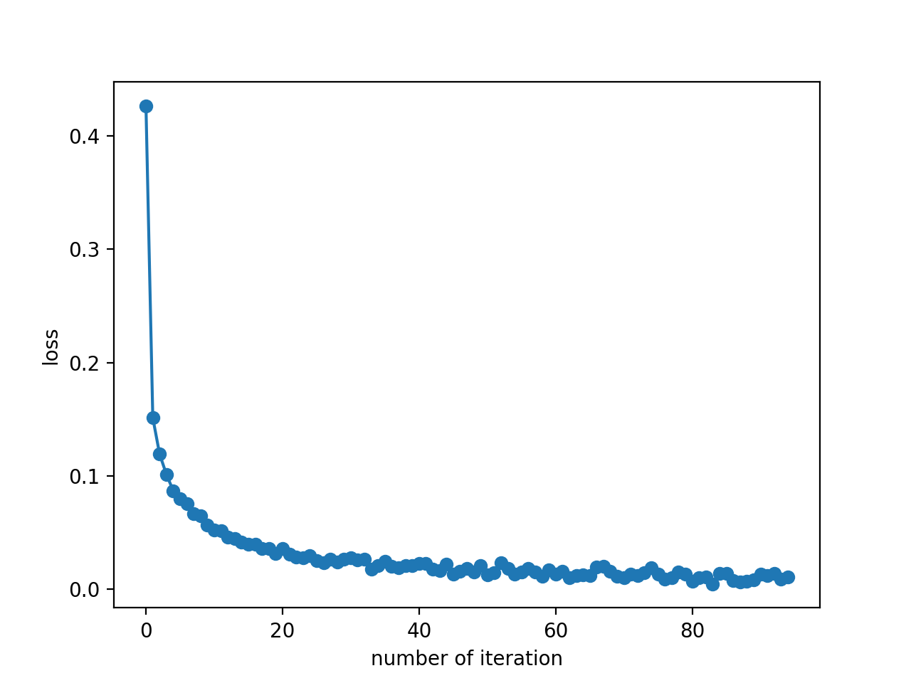 Figure 4: The evolution of the loss across the training iterations. Figure made by the author.
Here we see that the loss decreases really fast during training and it saturates after the
40th iteration (remember that we defined max 100 iterations as hyperparameter).
2.6 Visualizing the learnt weights
Here we need first to understand how the weights (learnt model parameters of each layer) are stored.
Based on the documentation, the attribute classifier.coefs_ is a list of shape (n_layers-1, )of weight arrays, where weight matrix at index i represents the weights between layer i and layer i+1. In this example, we defined 3 hidden layers and we also have the input and output layers. Thus, **** we expect to have 4 weight arrays for the between-layers weights (**in-L1, L1-L2, L2-L3**and**L2-out**in Figure 5).
Similarly, classifier.intercepts_is a list of bias vectors, where the vector at index i represents the bias values added to layer i+1.
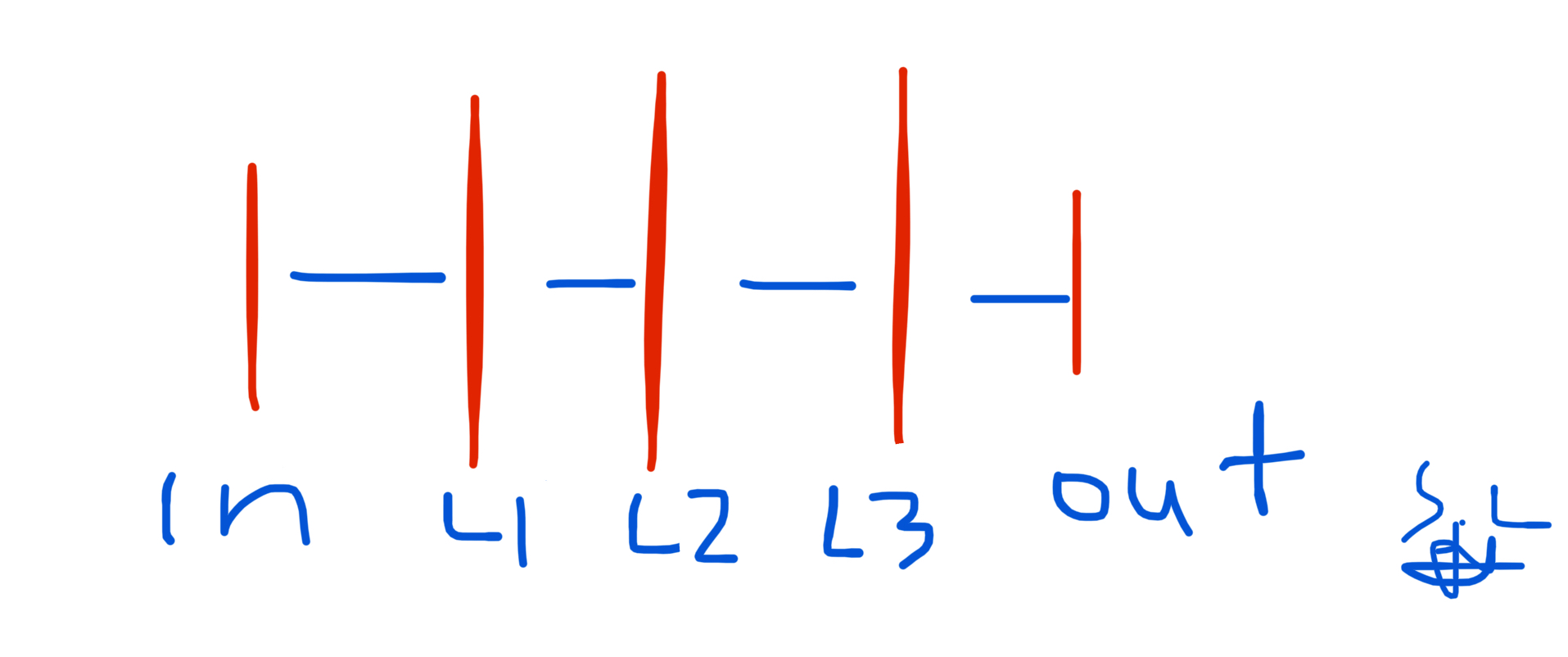 Figure 5: Handmade figure by the author on Notes (iOS).
Let's verify this:
text
len(classifier.intercepts_) == len(classifier.coefs_) == 4
correctly returns True.
Reminder: The input layer weight matrix will have shape 784 x #neurons_in_1st_hidden_layer. The output layer weight matrix will have shape #neurons_in_3rd_hidden_layer x #number_of_classes.
Visualizing the learnt weights of the input layer
text
target_layer = 0 #0 is input, 1 is 1st hidden etc
text
fig, axes = plt.subplots(1, 1, figsize=(15,6))
axes.imshow(np.transpose(classifier.coefs_[target_layer]), cmap=plt.get_cmap("gray"), aspect="auto")
text
axes.set_xlabel(f"number of neurons in {target_layer}")
axes.set_ylabel("neurons in output layer")
plt.show()
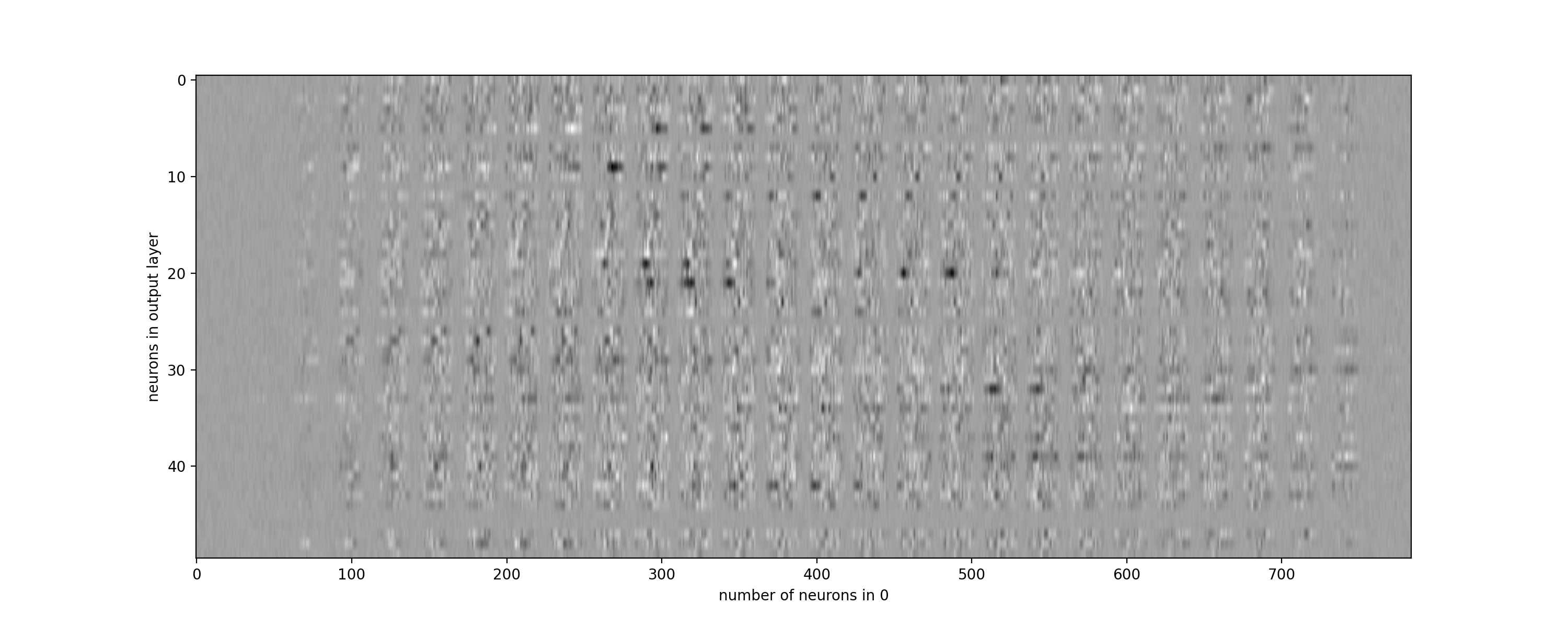 Figure 6: Visualization of the learnt weights of the neurons between the input and the 1st hidden layer. Figure made by the author.
Or reshape and plot them as 2D images again.
text
# choose layer to plot
target_layer = 0 #0 is input, 1 is 1st hidden etc
text
fig, axes = plt.subplots(4, 4)
vmin, vmax = classifier.coefs_[0].min(), classifier.coefs_[target_layer].max()
text
for coef, ax in zip(classifier.coefs_[0].T, axes.ravel()):
    ax.matshow(coef.reshape(28, 28), cmap=plt.cm.gray, vmin=0.5 * vmin, vmax=0.5 * vmax)
    ax.set_xticks(())
    ax.set_yticks(())
plt.show()
3. Summary
MLP classifier is a very powerful neural network model that enables the learning of non-linear functions for complex data. The method uses forward propagation to build the weights and then it computes the loss. Next, back propagation is used to update the weights so that the loss is reduced. This is done in an iterative way and the number of iterations is an input hyperparameter as I explained in the Introduction. Other important hyperparameters are the number of neurons in each hidden layer and the number of hidden layers in total. These need to be fine-tuned.
That's all folks! Hope you liked this article!
Stay tuned & support this effort
If you liked and found this article useful, follow me!
Questions? Post them as a comment and I will reply as soon as possible.
Latest posts
How to use Python & SQL to manipulate data in 1 min
Time-Series Forecasting: Predicting Stock Prices Using Facebook's Prophet Model
ROC Curve Explained using a COVID-19 hypothetical example: Binary & Multi-Class Classification...
Support Vector Machines (SVM) clearly explained: A python tutorial for classification problems...
Everything you need to know about Min-Max normalization in Python
How Scikit-Learn's StandardScaler works
References
[1] https://en.wikipedia.org/wiki/Multilayer_perceptron
[2] https://scikit-learn.org/stable/modules/neural_networks_supervised.html#mlp-tips
[3] https://scikit-learn.org/stable/modules/neural_networks_supervised.html#mathematical-formulation
[4] https://en.wikipedia.org/wiki/Backpropagation
[5] https://en.wikipedia.org/wiki/MNIST_database
Get in touch with me
Register Now to Continue Reading
Unlock Towards Data Science with a Free Account
All articles on Towards Data Science are available to registered users. Create a free account today to access this article and thousands more.
Register for freeSign in to your account
 Written By
See all from Serafeim Loukas, PhD
ClassificationMachine LearningMultilayer PerceptronNeural NetworksPerceptron
Share This Article
Towards Data Science is a community publication. Submit your insights to reach our global audience and earn through the TDS Author Payment Program.
Write for TDS
Related Articles
Artificial Intelligence
MultiMix: Sparingly Supervised, Extreme Multitask Learning from Medical Images
Ayaan Haque
June 9, 202217 min read
Large Language Models
Python implementation with machine learning classification, prompt engineering, feature engineering on text embedding and model...
Tony Zhang
July 13, 202311 min read
Deep Learning
How data symmetry informs neural network architectures
Caroline Arnold
April 30, 20253 min read
Machine Learning
How I improved speed by 10x
Anthony Cavin
June 28, 20227 min read
Artificial Intelligence
How to boost the performance with bagging and boosting
Soner Yıldırım
June 6, 20205 min read
Artificial Intelligence
How to create informative distribution plots
Soner Yıldırım
May 29, 20204 min read
Artificial Intelligence
How to make sure your data science project gets a good start
Shahwaiz
January 7, 20226 min read
Machine Learning
Why you shouldn't be ashamed to use Excel as a data scientist
Tyler Folkman
March 4, 20204 min read
Deep Learning
TicTacGPT for playing simple board games
Charlie O'Neill
September 8, 202330 min read
Your home for data science and AI. The world's leading publication for data science, data analytics, data engineering, machine learning, and artificial intelligence professionals.
Subscribe to Our NewsletterWrite For TDS•About•Advertise•Privacy Policy•Terms of Use
© Insight Media Group, LLC 2026•The New Stack•roadmap.sh•Creator Network
Recommended Articles
Close