保留正文与补采附件。源页面当前未重新核验;具体限制见交付清单。
 We value your privacy
We use cookies to enhance your browsing experience, serve personalised ads or content, and analyse our traffic. By clicking "Accept All", you consent to our use of cookies.
Customise Reject All Accept All
Customise Consent Preferences
 We use cookies to help you navigate efficiently and perform certain functions. You will find detailed information about all cookies under each consent category below.
The cookies that are categorised as "Necessary" are stored on your browser as they are essential for enabling the basic functionalities of the site. ... Show more
NecessaryAlways Active
Necessary cookies are required to enable the basic features of this site, such as providing secure log-in or adjusting your consent preferences. These cookies do not store any personally identifiable data.
-
Cookie
BCTempID
-
Duration
10 minutes
-
Description
No description available.
-
Cookie
__cf_bm
-
Duration
1 hour
-
Description
This cookie, set by Cloudflare, is used to support Cloudflare Bot Management.
-
Cookie
AWSALBCORS
-
Duration
7 days
-
Description
Amazon Web Services set this cookie for load balancing.
-
Cookie
_cfuvid
-
Duration
session
-
Description
Cloudflare sets this cookie to track users across sessions to optimize user experience by maintaining session consistency and providing personalized services
-
Cookie
li_gc
-
Duration
6 months
-
Description
Linkedin set this cookie for storing visitor's consent regarding using cookies for non-essential purposes.
-
Cookie
__hssrc
-
Duration
session
-
Description
This cookie is set by Hubspot whenever it changes the session cookie. The __hssrc cookie set to 1 indicates that the user has restarted the browser, and if the cookie does not exist, it is assumed to be a new session.
-
Cookie
__hssc
-
Duration
1 hour
-
Description
HubSpot sets this cookie to keep track of sessions and to determine if HubSpot should increment the session number and timestamps in the __hstc cookie.
-
Cookie
wpEmojiSettingsSupports
-
Duration
session
-
Description
WordPress sets this cookie when a user interacts with emojis on a WordPress site. It helps determine if the user's browser can display emojis properly.
-
Cookie
BCSessionID
-
Duration
1 year 1 month 4 days
-
Description
Blueconic sets this cookie as a unique identifier for the BlueConic profile.
-
Cookie
_octo
-
Duration
1 year
-
Description
No description available.
-
Cookie
logged_in
-
Duration
1 year
-
Description
No description available.
-
Cookie
__Secure-YEC
-
Duration
past
-
Description
YouTube sets this cookie to stores the user's video player preferences using embedded YouTube video
-
Cookie
__eoi
-
Duration
6 months
-
Description
Description is currently not available.
-
Cookie
AWSALBTGCORS
-
Duration
7 days
-
Description
No description available.
-
Cookie
login-status-p
-
Duration
past
-
Description
Description is currently not available.
-
Cookie
AWSALBTG
-
Duration
7 days
-
Description
No description available.
-
Cookie
csrf_token
-
Duration
session
-
Description
No description available.
-
Cookie
token_v2
-
Duration
1 day
-
Description
Description is currently not available.
-
Cookie
D
-
Duration
1 year
-
Description
Description is currently not available.
-
Cookie
PHPSESSID
-
Duration
session
-
Description
This cookie is native to PHP applications. The cookie stores and identifies a user's unique session ID to manage user sessions on the website. The cookie is a session cookie and will be deleted when all the browser windows are closed.
-
Cookie
VISITOR_PRIVACY_METADATA
-
Duration
6 months
-
Description
YouTube sets this cookie to store the user's cookie consent state for the current domain.
-
Cookie
cookietest
-
Duration
session
-
Description
The cookietest cookie is typically used to determine whether the user's browser accepts cookies, essential for website functionality and user experience.
-
Cookie
__Host-airtable-session
-
Duration
1 year
-
Description
This cookie is used to enable us to integrate the services of Airtable.
-
Cookie
__Host-airtable-session.sig
-
Duration
1 year
-
Description
This cookie is used to enable us to integrate the services of Airtable.
-
Cookie
m
-
Duration
1 year 1 month 4 days
-
Description
Stripe sets this cookie for fraud prevention purposes. It identifies the device used to access the website, allowing the website to be formatted accordingly.
-
Cookie
BIGipServer*
-
Duration
session
-
Description
Marketo sets this cookie to collect information about the user's online activity and build a profile about their interests to provide advertisements relevant to the user.
-
Cookie
__cfruid
-
Duration
session
-
Description
Cloudflare sets this cookie to identify trusted web traffic.
-
Cookie
_GRECAPTCHA
-
Duration
6 months
-
Description
Google Recaptcha service sets this cookie to identify bots to protect the website against malicious spam attacks.
-
Cookie
__Secure-YNID
-
Duration
6 months
-
Description
Google cookie used to protect user security and prevent fraud, especially during the login process.
-
Cookie
cookieyes-consent
-
Duration
1 year
-
Description
CookieYes sets this cookie to remember users' consent preferences so that their preferences are respected on subsequent visits to this site. It does not collect or store any personal information about the site visitors.
Functional
Functional cookies help perform certain functionalities like sharing the content of the website on social media platforms, collecting feedback, and other third-party features.
-
Cookie
lidc
-
Duration
1 day
-
Description
LinkedIn sets the lidc cookie to facilitate data center selection.
-
Cookie
brw
-
Duration
1 year
-
Description
No description available.
-
Cookie
brwConsent
-
Duration
5 minutes
-
Description
Description is currently not available.
-
Cookie
WMF-Uniq
-
Duration
1 year
-
Description
Description is currently not available.
-
Cookie
loom_anon_comment
-
Duration
1 year
-
Description
No description available.
-
Cookie
loom_referral_video
-
Duration
session
-
Description
Description is currently not available.
-
Cookie
VISITOR_INFO1_LIVE
-
Duration
6 months
-
Description
A cookie set by YouTube to measure bandwidth that determines whether the user gets the new or old player interface.
-
Cookie
yt-remote-connected-devices
-
Duration
Never Expires
-
Description
YouTube sets this cookie to store the user's video preferences using embedded YouTube videos.
-
Cookie
ytidb::LAST_RESULT_ENTRY_KEY
-
Duration
Never Expires
-
Description
The cookie ytidb::LAST_RESULT_ENTRY_KEY is used by YouTube to store the last search result entry that was clicked by the user. This information is used to improve the user experience by providing more relevant search results in the future.
-
Cookie
yt-remote-device-id
-
Duration
Never Expires
-
Description
YouTube sets this cookie to store the user's video preferences using embedded YouTube videos.
-
Cookie
yt-remote-session-name
-
Duration
session
-
Description
The yt-remote-session-name cookie is used by YouTube to store the user's video player preferences using embedded YouTube video.
-
Cookie
yt-remote-fast-check-period
-
Duration
session
-
Description
The yt-remote-fast-check-period cookie is used by YouTube to store the user's video player preferences for embedded YouTube videos.
-
Cookie
yt-remote-session-app
-
Duration
session
-
Description
The yt-remote-session-app cookie is used by YouTube to store user preferences and information about the interface of the embedded YouTube video player.
-
Cookie
yt-remote-cast-available
-
Duration
session
-
Description
The yt-remote-cast-available cookie is used to store the user's preferences regarding whether casting is available on their YouTube video player.
-
Cookie
yt-remote-cast-installed
-
Duration
session
-
Description
The yt-remote-cast-installed cookie is used to store the user's video player preferences using embedded YouTube video.
-
Cookie
cp_session
-
Duration
3 months
-
Description
Codepen sets this cookie for Help systems found in the website.
-
Cookie
loid
-
Duration
1 year 1 month 4 days
-
Description
This cookie is set by the Reddit. The cookie enables the sharing of content from the website onto the social media platform.
Analytics
Analytical cookies are used to understand how visitors interact with the website. These cookies help provide information on metrics such as the number of visitors, bounce rate, traffic source, etc.
-
Cookie
__hstc
-
Duration
6 months
-
Description
Hubspot set this main cookie for tracking visitors. It contains the domain, initial timestamp (first visit), last timestamp (last visit), current timestamp (this visit), and session number (increments for each subsequent session).
-
Cookie
hubspotutk
-
Duration
6 months
-
Description
HubSpot sets this cookie to keep track of the visitors to the website. This cookie is passed to HubSpot on form submission and used when deduplicating contacts.
-
Cookie
_ga
-
Duration
1 year 1 month 4 days
-
Description
Google Analytics sets this cookie to calculate visitor, session and campaign data and track site usage for the site's analytics report. The cookie stores information anonymously and assigns a randomly generated number to recognise unique visitors.
-
Cookie
ga*
-
Duration
1 year 1 month 4 days
-
Description
Google Analytics sets this cookie to store and count page views.
-
Cookie
__Host-psifi.analyticsTrace
-
Duration
6 hours
-
Description
Description is currently not available.
-
Cookie
__Host-psifi.analyticsTraceV2
-
Duration
6 hours
-
Description
Description is currently not available.
-
Cookie
_gh_sess
-
Duration
session
-
Description
GitHub sets this cookie for temporary application and framework state between pages like what step the user is on in a multiple step form.
-
Cookie
YSC
-
Duration
session
-
Description
YSC cookie is set by Youtube and is used to track the views of embedded videos on Youtube pages.
-
Cookie
ajs_anonymous_id
-
Duration
1 year
-
Description
This cookie is set by Segment to count the number of people who visit a certain site by tracking if they have visited before.
-
Cookie
vuid
-
Duration
1 year 1 month 4 days
-
Description
Vimeo installs this cookie to collect tracking information by setting a unique ID to embed videos on the website.
Performance
Performance cookies are used to understand and analyse the key performance indexes of the website which helps in delivering a better user experience for the visitors.
-
Cookie
AWSALB
-
Duration
7 days
-
Description
AWSALB is an application load balancer cookie set by Amazon Web Services to map the session to the target.
-
Cookie
acq
-
Duration
past
-
Description
Description is currently not available.
-
Cookie
acq.sig
-
Duration
past
-
Description
Description is currently not available.
-
Cookie
ptc
-
Duration
2 years
-
Description
No description available.
Advertisement
Advertisement cookies are used to provide visitors with customised advertisements based on the pages you visited previously and to analyse the effectiveness of the ad campaigns.
-
Cookie
muc_ads
-
Duration
1 year 1 month 4 days
-
Description
Twitter sets this cookie to collect user behaviour and interaction data to optimize the website.
-
Cookie
guest_id_marketing
-
Duration
1 year 1 month 4 days
-
Description
Twitter sets this cookie to identify and track the website visitor.
-
Cookie
guest_id_ads
-
Duration
1 year 1 month 4 days
-
Description
Twitter sets this cookie to identify and track the website visitor.
-
Cookie
personalization_id
-
Duration
1 year 1 month 4 days
-
Description
Twitter sets this cookie to integrate and share features for social media and also store information about how the user uses the website, for tracking and targeting.
-
Cookie
guest_id
-
Duration
1 year 1 month 4 days
-
Description
Twitter sets this cookie to identify and track the website visitor. It registers if a user is signed in to the Twitter platform and collects information about ad preferences.
-
Cookie
bcookie
-
Duration
1 year
-
Description
LinkedIn sets this cookie from LinkedIn share buttons and ad tags to recognize browser IDs.
-
Cookie
__Secure-ROLLOUT_TOKEN
-
Duration
6 months
-
Description
YouTube sets this cookie to manage feature rollout and experimentation. It helps Google control which new features or interface changes are shown to users as part of testing and staged rollouts, ensuring consistent experience for a given user during an experiment.
-
Cookie
yt.innertube::nextId
-
Duration
Never Expires
-
Description
YouTube sets this cookie to register a unique ID to store data on what videos from YouTube the user has seen.
-
Cookie
yt.innertube::requests
-
Duration
Never Expires
-
Description
YouTube sets this cookie to register a unique ID to store data on what videos from YouTube the user has seen.
-
Cookie
session_tracker
-
Duration
session
-
Description
This cookie is set by the Reddit. This cookie is used to identify trusted web traffic. It also helps in adverstising on the website.
-
Cookie
edgebucket
-
Duration
session
-
Description
Reddit sets this cookie to save the information about a log-on Reddit user, for the purpose of advertisement recommendations and updating the content.
-
Cookie
did
-
Duration
1 year
-
Description
Arbor sets this cookie to show targeted ads to site visitors.This cookie expires after 2 months or 1 year.
Uncategorised
Other uncategorised cookies are those that are being analysed and have not been classified into a category as yet.
No cookies to display.
Reject All Save My Preferences Accept All
Toggle SearchToggle Mobile Navigation
Publish AI, ML & data-science insights to a global community of data professionals.
Sign inSubmit an Article
LatestEditor's PicksNewsletterShipAI
Write For TDS
LinkedInXToggle Search
Efficient Image Segmentation Using PyTorch: Part 3
Depthwise separable convolutions
Dhruv Matani
June 27, 202313 min read
In this 4-part series, we'll implement image segmentation step by step from scratch using deep learning techniques in PyTorch. This part will focus on optimizing our CNN baseline model using depthwise separable convolutions to reduce the number of trainable parameters, making the model deployable on mobile and other edge devices.
Co-authored with Naresh Singh
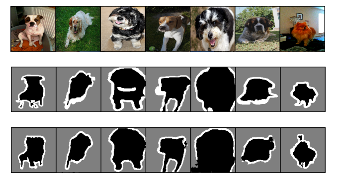 Figure 1: Result of running image segmentation using a CNN with depth-wise separable convolutions instead of regular convolutions. From top to bottom, input images, ground truth segmentation masks, and predicted segmentation masks. Source: Author(s)
Article outline
In this article, we will augment the Convolutional Neural Network (CNN) we built earlier to reduce the number of learnable parameters in our network. The task of identifying pet pixels (pixels belonging to cats, dogs, hamsters, etc...) in an input image remains unchanged. Our network of choice will remain SegNet, and the only change we'll make is to replace our convolutional layers with depth-wise-separable-convolutions (DSC). Before we do this, we will dive into the theory and practice of depth-wise-separable-convolutions, and appreciate the idea behind the technique.
Throughout this article, we will reference code and results from this [notebook](https://github.com/dhruvbird/ml-notebooks/blob/main/pets_segmentation/oxford-iiit-pets-segmentation-using-pytorch-segnet-and-depth-wise-separable-convs.ipynb) for model training, and this notebook for a primer on DSC. If you wish to reproduce the results, you'll need a GPU to ensure that the first notebook completes running in a reasonable amount of time. The second notebook can be run on a regular CPU.
Articles in this series
This series is for readers at all experience levels with deep learning. If you want to learn about the practice of deep learning and vision AI along with some solid theory and hands-on experience, you've come to the right place! This is expected to be a 4-part series with the following articles:
- Concepts and Ideas
- A CNN-based model
- Depthwise separable convolutions (this article)
- A Vision Transformer-based model
Introduction
Let's start this discussion with a closer look at the convolutions from the perspective of model size and computation cost. The number of trainable parameters is a good indication of the size of a model and the number of the tensor operations reflects the model complexity or computation cost. Consider that we have a convolution layer with n filters with size dₖ x dₖ. Further assume that this layer processes input with shape m x h x w, where m is the number of input channels, and h and w are height and width dimensions respectively. In this case, the convolution layer will produce an output with shape n x h x w as shown in Figure 2. We are assuming that the convolution uses stride=1. Let's go ahead and evaluate this setup in terms of trainable parameters and computation cost.
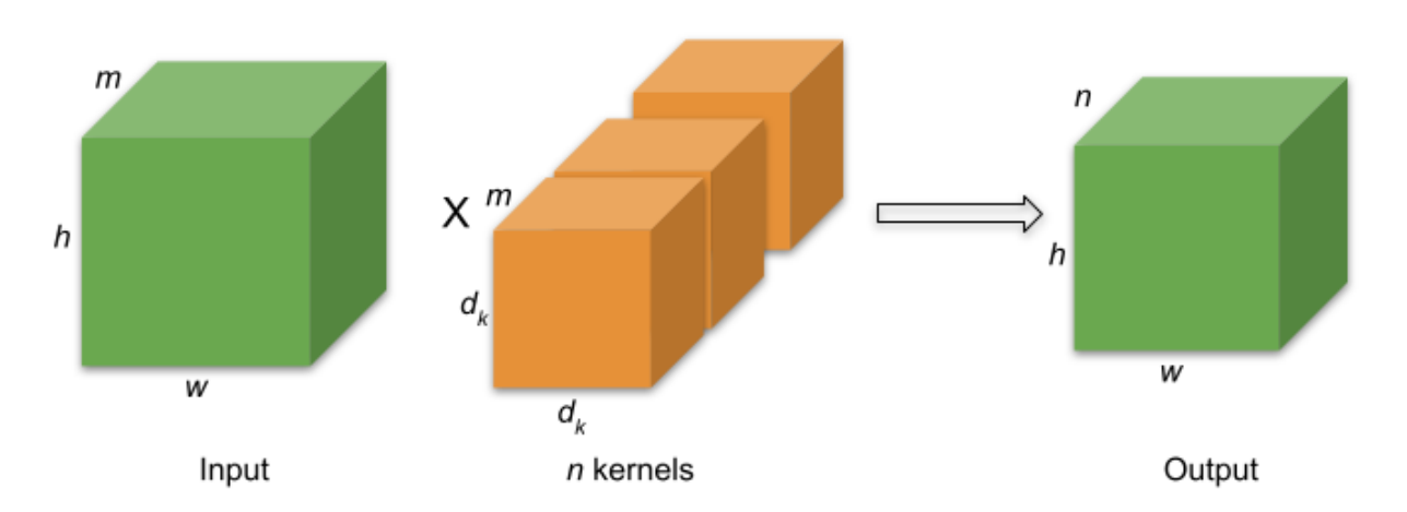 Figure 2: Regular convolutional filters applied to input to produce output. Assume stride=1 and padding=dₖ-2. Source: Efficient Deep Learning Book
Evaluation Of Trainable Parameters: We have n filters, each of which has m x dₖ x dₖ learnable parameters. This results in a total of n x m x dₖ x dₖ learnable parameters. Bias terms are ignored to simplify this discussion. Let's look at the PyTorch code below to validate our understanding.
python
import torch
from torch import nn
def num_parameters(m):
return sum([p.numel() for p in m.parameters()])
dk, m, n = 3, 16, 32
print(f"Expected number of parameters: {m * dk * dk * n}")
conv1 = nn.Conv2d(in_channels=m, out_channels=n, kernel_size=dk, bias=False)
print(f"Actual number of parameters: {num_parameters(conv1)}")
Prints the following.
text
Expected number of parameters: 4608
Actual number of parameters: 4608
Now, let's evaluate the computation costs of convolution.
Evaluation Of Computational Cost: A single convolutional filter of shape m x dₖ x dₖ when run with a stride=1 and a padding=dₖ-2 on an input with size h x w will apply the convolutional filter h x w times, once for each image section with size dₖ x dₖ amounting to a total of h x w sections. It results in a cost of m x dₖ x dₖ x h x w per filter or output channel. Since we wish to compute n output channels, the total cost will be m x dₖ x dₖ x h x n. Let's go ahead and validate this using the torchinfo PyTorch package.
python
from torchinfo import summary
h, w = 128, 128
print(f"Expected total multiplies: {m * dk * dk * h * w * n}")
summary(conv1, input_size=(1, m, h, w))
Will print the following.
text
Expected total multiplies: 75497472

==========================================================================================
Layer (type:depth-idx)                   Output Shape              Param #
==========================================================================================
Conv2d                                   [1, 32, 128, 128]         4,608
==========================================================================================
Total params: 4,608
Trainable params: 4,608
Non-trainable params: 0
Total mult-adds (M): 75.50
==========================================================================================
Input size (MB): 1.05
Forward/backward pass size (MB): 4.19
Params size (MB): 0.02
Estimated Total Size (MB): 5.26
==========================================================================================
If we ignore the implementation details of a convolution layer for a moment, we would realize that, on a high level, a convolution layer just transforms a m x h x w input into a n x h x w output. The transformation is achieved through trainable filters which progressively learn features as they see inputs. The question that follows is: Is it possible to achieve this transformation using fewer learnable parameters and simultaneously ensuring minimum compromise in the learning capabilities of the layer? Depthwise Separable Convolutions were proposed to answer this exact question. Let's understand them in detail and learn how they stack up on our evaluation metrics.
Depthwise Separable Convolution
The concept of Depthwise Separable Convolutions (DSC) was first proposed by Laurent Sifre in their PhD thesis titled Rigid-Motion Scattering For Image Classification. Since then, they have been used successfully in various popular deep convolutional networks such as XceptionNet and MobileNet.
The main difference between a regular convolution, and a DSC is that a DSC is composed of 2 convolutions as described below:
- A depthwise grouped convolution , where the number of input channels m is equal to the number of output channels such that each output channel is affected only by a single input channel. In PyTorch, this is called a "grouped" convolution. You can read more about grouped convolutions in PyTorch here.
- A pointwise convolution (filter size=1), which operates like a regular convolution such that each of the n filters operates on all m input channels to produce a single output value.
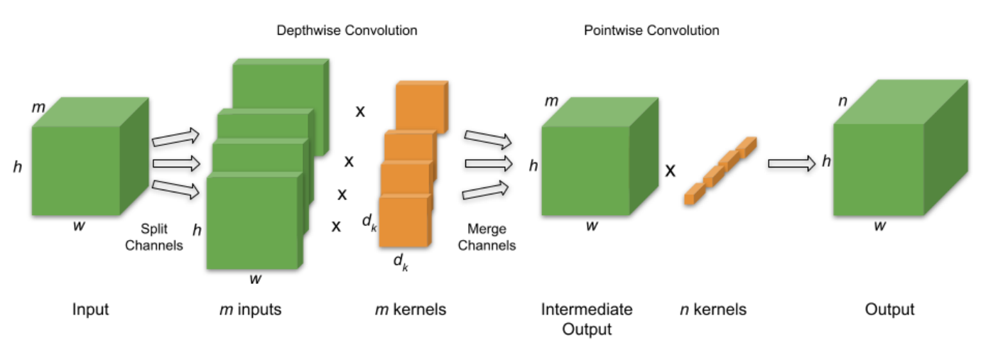 Figure 3: Depthwise Separable Convolution filters applied to input to produce output. Assume stride=1 and padding=dₖ-2. Source: Efficient Deep Learning Book
Let's perform the same exercise that we did for regular convolutions for DSCs and compute the number of trainable parameters and computations.
Evaluation Of Trainable Parameters: The "grouped" convolutions have m filters, each of which has dₖ x dₖ learnable parameters which produces m output channels. This results in a total of m x dₖ x dₖ learnable parameters. The pointwise convolution has n filters of size m x 1 x 1 which adds up to n x m x 1 x 1 learnable parameters. Let's look at the PyTorch code below to validate our understanding.
python
class DepthwiseSeparableConv(nn.Sequential):
    def __init__(self, chin, chout, dk):
        super().__init__(
            # Depthwise convolution
            nn.Conv2d(chin, chin, kernel_size=dk, stride=1, padding=dk-2, bias=False, groups=chin),
            # Pointwise convolution
            nn.Conv2d(chin, chout, kernel_size=1, bias=False),
        )

conv2 = DepthwiseSeparableConv(chin=m, chout=n, dk=dk)
print(f"Expected number of parameters: {m * dk * dk + m * 1 * 1 * n}")
print(f"Actual number of parameters: {num_parameters(conv2)}")
Which will print.
text
Expected number of parameters: 656
Actual number of parameters: 656
We can see that the DSC version has roughly 7x less parameters. Next, let's focus our attention on the computation costs for a DSC layer.
Evaluation Of Computational Cost: Let's assume our input has spatial dimensions m x h x w. In the grouped convolution segment of DSC, we have m filters, each with size dₖ x dₖ. A filter is applied to its corresponding input channel resulting in the segment cost of m x dₖ x dₖ x h x w. For the pointwise convolution, we apply n filters of size m x 1 x 1 **** to produce** n** output channels. This results in the segment cost of n x m x 1 x 1 x h x w. We need to add up the costs of the grouped and pointwise operations to compute the total cost. Let's go ahead and validate this using the torchinfo PyTorch package.
python
print(f"Expected total multiplies: {m * dk * dk * h * w + m * 1 * 1 * h * w * n}")
s2 = summary(conv2, input_size=(1, m, h, w))
print(f"Actual multiplies: {s2.total_mult_adds}")
print(s2)
Which will print.
text
Expected total multiplies: 10747904
Actual multiplies: 10747904
==========================================================================================
Layer (type:depth-idx)                   Output Shape              Param #
==========================================================================================
DepthwiseSeparableConv                   [1, 32, 128, 128]         --
├─Conv2d: 1-1                            [1, 16, 128, 128]         144
├─Conv2d: 1-2                            [1, 32, 128, 128]         512
==========================================================================================
Total params: 656
Trainable params: 656
Non-trainable params: 0
Total mult-adds (M): 10.75
==========================================================================================
Input size (MB): 1.05
Forward/backward pass size (MB): 6.29
Params size (MB): 0.00
Estimated Total Size (MB): 7.34
==========================================================================================
Let's compare the sizes and costs of both the convolutions for a few examples to gain some intuition.
Size and Cost comparison for regular and depthwise separable convolutions
To compare the size and cost of regular and depthwise separable convolution, we will assume an input size of 128 x 128 to the network, a kernel size of 3 x 3 , and a network that progressively halves the spatial dimensions and doubles the number of channel dimensions. We assume a single 2d-conv layer at every step, but in practice, there could be more.
 Figure 4: Comparing the number of trainable parameters (size) and multi-adds (cost) of regular and depthwise separable convolutions. We also show the ratio of the size and cost for the 2 types of convolutions. Source: Author(s).
You can see that on average both the size and computational cost of DSC is about 11% to 12% of the cost of regular convolutions for the configuration mentioned above.
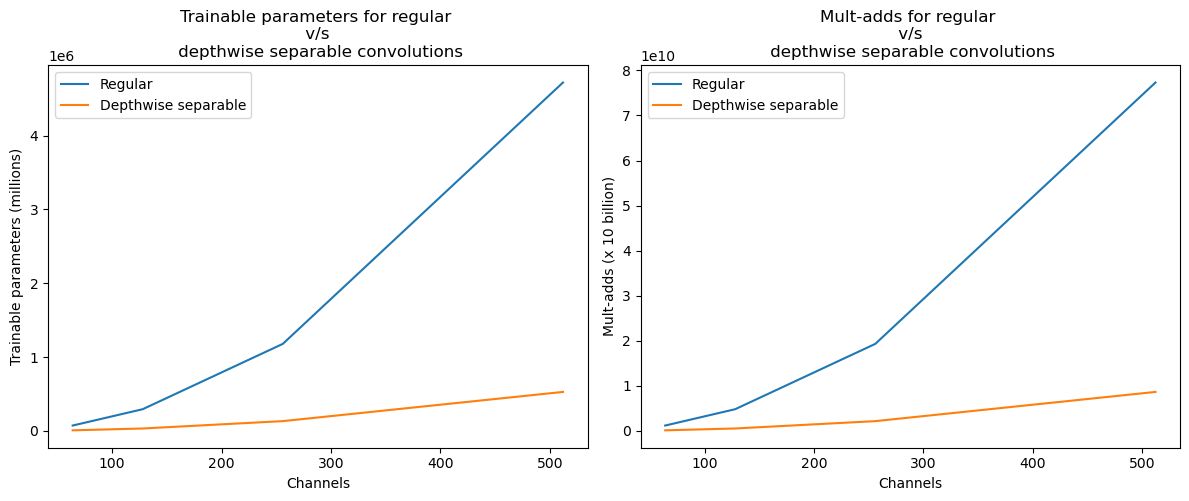 Figure 5: Relative size and cost of regular v/s DSC. Source: Author(s).
Now that we have developed a good understanding of the types of convolutions and their relative costs, you must be wondering if there's any downside of using DSCs. Everything we've seen so far seems to suggest that they are better in every way! Well, we haven't yet considered an important aspect which is the impact they have on the accuracy of our model. Let's dive into it via an experiment below.
SegNet Using Depthwise Separable Convolutions
This notebook contains all the code for this section.
We will adapt our SegNet model from the previous post and replace all the regular convolutional layers with a DSC layer. Once we do this, we notice that the number of parameters in our notebook drops from 15.27M to 1.75M parameters, which is a reduction of 88.5%! This is inline with our earlier estimates of an 11% to 12% reduction in the number of trainable parameters of the network.
A similar configuration as before was used during model training and validation. The configuration is specified below.
- The random horizontal flip and colour jitter data augmentations are applied to the training set to prevent overfitting
- The images are resized to 128x128 pixels in a non-aspect preserving resize operation
- No input normalization is applied to the images - instead a batch normalization layer is used as the first layer of the model
- The model is trained for 20 epochs using the Adam optimizer with a LR of 0.001 and no LR scheduler
- The cross-entropy loss function is used to classify a pixel as belonging to a pet, the background, or a pet border
The model achieved a validation accuracy of 86.96% after 20 training epochs. This is less than the 88.28% accuracy achieved by the model using regular convolutions for the same number of training epochs. We have determined experimentally that training for more epochs improves the accuracy of both models, so 20 epochs is definitely not the end of the training cycle. We stop at 20 epochs for the purposes of this article for demonstration purposes.
We plotted a gif showing how the model is learning to predict the segmentation masks for 21 images in the validation set.
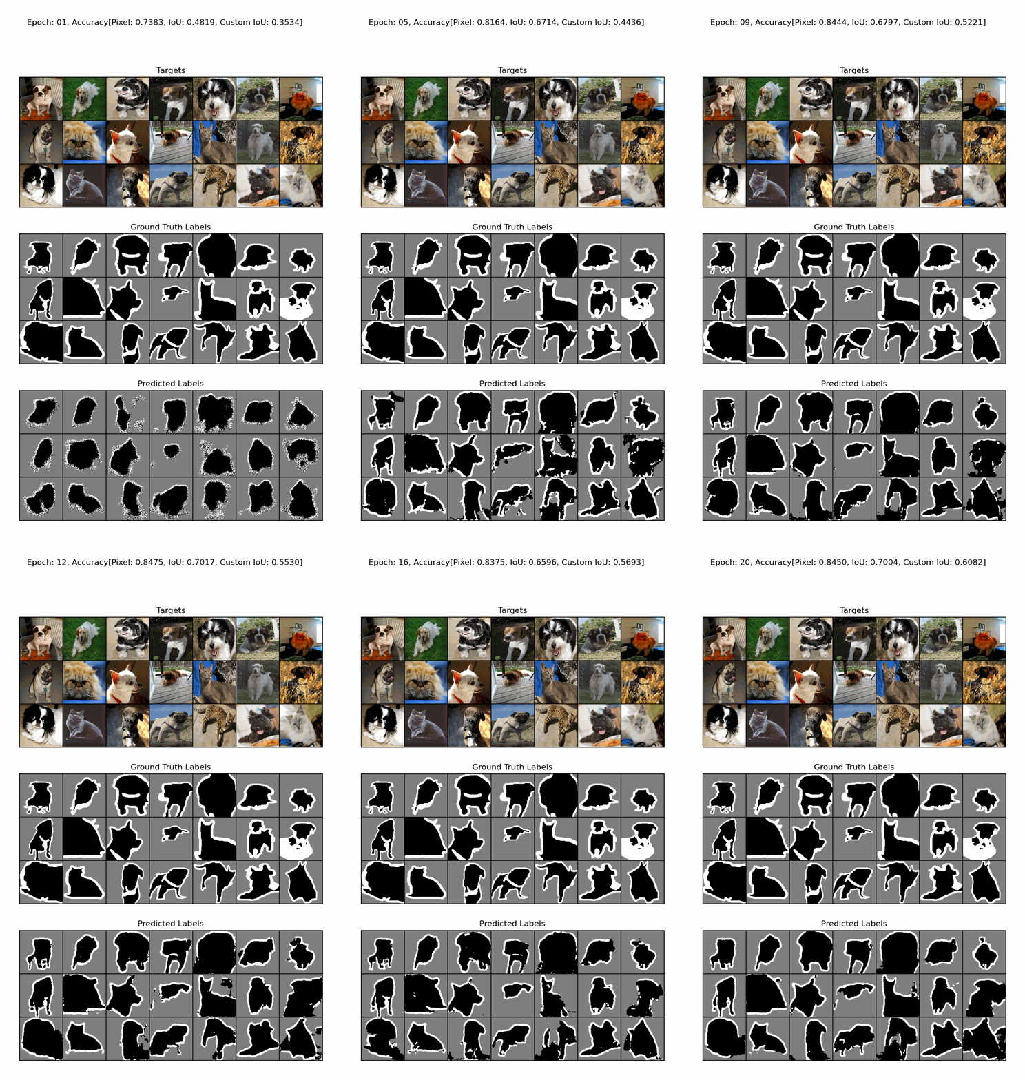 Figure 6: A gif showing how the SegNet model with DSC is learning to predict segmentation masks for 21 images in the validation set. Source: Author(s)
Now that we have seen how the model progresses through the training cycle, let's compare the train cycles of models with regular convolutions and DSC.
Accuracy Comparisons
We found it useful to look at the training cycles of the models using regular convolutions and DSC. The main difference we noticed is in the early phases (epochs) of training, after which both models settled roughly into the same prediction flow. In fact after training both models for 100 epochs, we noticed that the accuracy of the model with DSC is just about 1% less than the model with regular convolutions. This is inline with our observations from just 20 epochs of training.
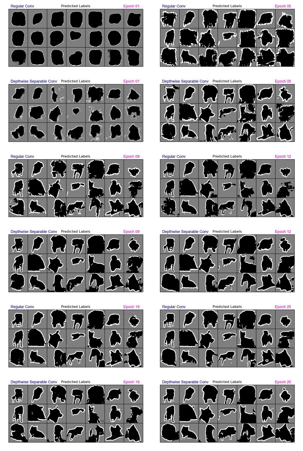 Figure 7: A gif showing the progression of segmentation masks predicted by the SegNet model using regular convolutions v/s DSC. Source: Author(s).
You would have noticed that both models get the predictions roughly right after just 6 training epochs - i.e. one can visually see that the models are predicting something useful. Most of the hard work of training the model is then above ensuring that the borders of the predicted masks are as tight as possible and as close to the actual pets in the image as possible. This means that while one can expect a lesser absolute increase in accuracy in the later training epochs, the impact of this on the quality of predictions is much more. We've noticed that a single digit of accuracy improvement at higher absolute accuracy values (going from 89% to 90%) results in significant qualitative improvements to the predictions.
Comparison with a UNet model
We ran an experiment that changed a lot of hyperparameters with a focus on improving the overall accuracy to get a sense of how far this setting is from close to optimal. Here's the configuration of that experiment.
- Image size: 128 x 128 - same as the experiments so far
- Train epochs: 100 - current experiments trained for 20 epochs
- Augmentations: A lot more augmentations such as image rotation, channel dropping, random block removal. We used Albumentations instead of torchvision transforms. Albumentations automatically transforms segmentation masks for us
- LR Scheduler: A StepLR scheduler was used with a decay of 0.8x every 25 train epochs
- Loss function: We tried 4 different loss functions: Cross Entropy, Focal, Dice, Weighted Cross Entropy. Dice performed worst whereas the rest were pretty much comparable to each other. In fact the difference in best accuracy between the rest after 100 epochs was in the 4th digit after the decimal (assuming the accuracy is a number between 0.0 and 1.0)
- Convolution type: Regular
- Model type: UNet - current experiments used a SegNet model
We achieved a best validation accuracy of 91.3% for the setting above. We noticed that the image size significantly impacts the best validation accuracy. For example, when we changed the image size to 256 x 256, the best validation accuracy went up to 93.0%. However, training took much longer, and used more memory, which meant that we had to reduce the batch size.
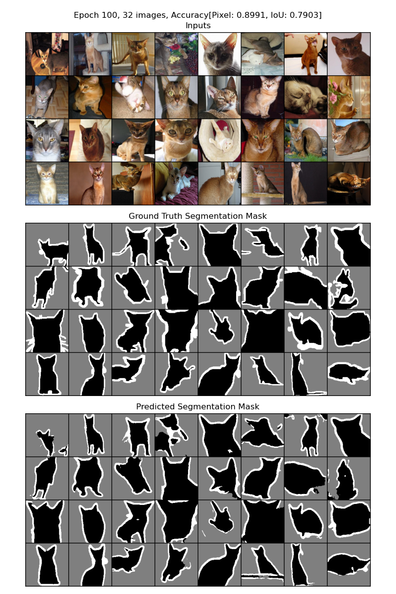 Figure 8: Result of training a UNet model for 100 train epochs with the hyperparameters mentioned above. Source: Author(s).
You can see that the predictions are much smoother and crisper compared to the ones we have been seeing so far.
Conclusion
In part-3 of this series, we learned about depth wise separable convolutions (DSC) as a technique to reduce model size and training/inference cost without a significant loss in validation accuracy. We learned about the size/cost tradeoff to expect between regular and DSC for a specific setting.
We showed how to adapt the SegNet model to use DSC in PyTorch. This technique can be applied to any deep CNN. In fact we can selectively replace some of the convolutional layers with DSC - i.e. we don't need to necessarily replace all of them. Choosing which layers to replace will depend on the balance you wish to strike between model size/runtime-cost and prediction accuracy. This decision will depend on your specific use case and deployment setup.
While this article trained models for 20 epochs, we explained that this is insufficient for production workloads, and provided a glimpse into what one can expect if one trains the model for more epochs. In addition, we provided an introduction to some of the hyperparameters that one can tune during model training. While this list is by no means comprehensive, it should allow you to appreciate the complexity and decision making needed to train an image segmentation model for production workloads.
In the next part of this series, we'll take a look at Vision Transformers, and how we can use this model architecture to perform image segmentation for the pets segmentation task.
References and further reading
Register Now to Continue Reading
Unlock Towards Data Science with a Free Account
All articles on Towards Data Science are available to registered users. Create a free account today to access this article and thousands more.
Register for freeSign in to your account
 Written By
See all from Dhruv Matani
CnnDepthwise ConvolutionPytorchPytorch Image SegmentSegnet
Share This Article
Towards Data Science is a community publication. Submit your insights to reach our global audience and earn through the TDS Author Payment Program.
Write for TDS
Related Articles
Data Science
Time series classification is a general problem that can be seen in many domains and contexts, e.g. for given time series of a financial...
Shuyang Xiang
November 20, 20214 min read
Technology
And get our hands dirty by formulating a Node Classification task using DGL, PyG and Spektral.
Rohith Teja
August 21, 20215 min read
How to leverage a powerful pre-trained convolution neural network to extract embedding vectors for pictures.
Gianmario Spacagna
December 2, 20207 min read
Machine Learning
Train state-of-the-art speech recognition, NLP and TTS models at scale with NeMo and Lightning
Sean Narenthiran
October 28, 20204 min read
Deep Learning has taken over vision, natural language processing, speech recognition, and many other fields achieving astonishing results...
Samrat Thapa
October 23, 20207 min read
Deep Learning
PyTorch Model Performance Analysis and Optimization - Part 4
Chaim Rand
August 26, 202311 min read
Artificial Intelligence
Hiding host-device synchronization via CUDA stream interleaving
Chaim Rand
February 24, 202615 min read
Deep Learning
Pytorch has a great ecosystem to load custom datasets for training machine learning models. This is the first part of the two-part series...
Utkarsh Garg
August 18, 20215 min read
Deep Learning
A deep dive into PyTorch DataLoader with Multiprocessing
Mengliu Zhao
June 2, 20246 min read
Your home for data science and AI. The world's leading publication for data science, data analytics, data engineering, machine learning, and artificial intelligence professionals.
Subscribe to Our NewsletterWrite For TDS•About•Advertise•Privacy Policy•Terms of Use
© Insight Media Group, LLC 2026•The New Stack•roadmap.sh•Creator Network
Recommended Articles
Close