保留正文与补采附件。源页面当前未重新核验;具体限制见交付清单。
 We value your privacy
We use cookies to enhance your browsing experience, serve personalised ads or content, and analyse our traffic. By clicking "Accept All", you consent to our use of cookies.
Customise Reject All Accept All
Customise Consent Preferences
 We use cookies to help you navigate efficiently and perform certain functions. You will find detailed information about all cookies under each consent category below.
The cookies that are categorised as "Necessary" are stored on your browser as they are essential for enabling the basic functionalities of the site. ... Show more
NecessaryAlways Active
Necessary cookies are required to enable the basic features of this site, such as providing secure log-in or adjusting your consent preferences. These cookies do not store any personally identifiable data.
-
Cookie
BCTempID
-
Duration
10 minutes
-
Description
No description available.
-
Cookie
__cf_bm
-
Duration
1 hour
-
Description
This cookie, set by Cloudflare, is used to support Cloudflare Bot Management.
-
Cookie
AWSALBCORS
-
Duration
7 days
-
Description
Amazon Web Services set this cookie for load balancing.
-
Cookie
_cfuvid
-
Duration
session
-
Description
Cloudflare sets this cookie to track users across sessions to optimize user experience by maintaining session consistency and providing personalized services
-
Cookie
li_gc
-
Duration
6 months
-
Description
Linkedin set this cookie for storing visitor's consent regarding using cookies for non-essential purposes.
-
Cookie
__hssrc
-
Duration
session
-
Description
This cookie is set by Hubspot whenever it changes the session cookie. The __hssrc cookie set to 1 indicates that the user has restarted the browser, and if the cookie does not exist, it is assumed to be a new session.
-
Cookie
__hssc
-
Duration
1 hour
-
Description
HubSpot sets this cookie to keep track of sessions and to determine if HubSpot should increment the session number and timestamps in the __hstc cookie.
-
Cookie
wpEmojiSettingsSupports
-
Duration
session
-
Description
WordPress sets this cookie when a user interacts with emojis on a WordPress site. It helps determine if the user's browser can display emojis properly.
-
Cookie
BCSessionID
-
Duration
1 year 1 month 4 days
-
Description
Blueconic sets this cookie as a unique identifier for the BlueConic profile.
-
Cookie
_octo
-
Duration
1 year
-
Description
No description available.
-
Cookie
logged_in
-
Duration
1 year
-
Description
No description available.
-
Cookie
__Secure-YEC
-
Duration
past
-
Description
YouTube sets this cookie to stores the user's video player preferences using embedded YouTube video
-
Cookie
__eoi
-
Duration
6 months
-
Description
Description is currently not available.
-
Cookie
AWSALBTGCORS
-
Duration
7 days
-
Description
No description available.
-
Cookie
login-status-p
-
Duration
past
-
Description
Description is currently not available.
-
Cookie
AWSALBTG
-
Duration
7 days
-
Description
No description available.
-
Cookie
csrf_token
-
Duration
session
-
Description
No description available.
-
Cookie
token_v2
-
Duration
1 day
-
Description
Description is currently not available.
-
Cookie
D
-
Duration
1 year
-
Description
Description is currently not available.
-
Cookie
PHPSESSID
-
Duration
session
-
Description
This cookie is native to PHP applications. The cookie stores and identifies a user's unique session ID to manage user sessions on the website. The cookie is a session cookie and will be deleted when all the browser windows are closed.
-
Cookie
VISITOR_PRIVACY_METADATA
-
Duration
6 months
-
Description
YouTube sets this cookie to store the user's cookie consent state for the current domain.
-
Cookie
cookietest
-
Duration
session
-
Description
The cookietest cookie is typically used to determine whether the user's browser accepts cookies, essential for website functionality and user experience.
-
Cookie
__Host-airtable-session
-
Duration
1 year
-
Description
This cookie is used to enable us to integrate the services of Airtable.
-
Cookie
__Host-airtable-session.sig
-
Duration
1 year
-
Description
This cookie is used to enable us to integrate the services of Airtable.
-
Cookie
m
-
Duration
1 year 1 month 4 days
-
Description
Stripe sets this cookie for fraud prevention purposes. It identifies the device used to access the website, allowing the website to be formatted accordingly.
-
Cookie
BIGipServer*
-
Duration
session
-
Description
Marketo sets this cookie to collect information about the user's online activity and build a profile about their interests to provide advertisements relevant to the user.
-
Cookie
__cfruid
-
Duration
session
-
Description
Cloudflare sets this cookie to identify trusted web traffic.
-
Cookie
_GRECAPTCHA
-
Duration
6 months
-
Description
Google Recaptcha service sets this cookie to identify bots to protect the website against malicious spam attacks.
-
Cookie
__Secure-YNID
-
Duration
6 months
-
Description
Google cookie used to protect user security and prevent fraud, especially during the login process.
-
Cookie
cookieyes-consent
-
Duration
1 year
-
Description
CookieYes sets this cookie to remember users' consent preferences so that their preferences are respected on subsequent visits to this site. It does not collect or store any personal information about the site visitors.
Functional
Functional cookies help perform certain functionalities like sharing the content of the website on social media platforms, collecting feedback, and other third-party features.
-
Cookie
lidc
-
Duration
1 day
-
Description
LinkedIn sets the lidc cookie to facilitate data center selection.
-
Cookie
brw
-
Duration
1 year
-
Description
No description available.
-
Cookie
brwConsent
-
Duration
5 minutes
-
Description
Description is currently not available.
-
Cookie
WMF-Uniq
-
Duration
1 year
-
Description
Description is currently not available.
-
Cookie
loom_anon_comment
-
Duration
1 year
-
Description
No description available.
-
Cookie
loom_referral_video
-
Duration
session
-
Description
Description is currently not available.
-
Cookie
VISITOR_INFO1_LIVE
-
Duration
6 months
-
Description
A cookie set by YouTube to measure bandwidth that determines whether the user gets the new or old player interface.
-
Cookie
yt-remote-connected-devices
-
Duration
Never Expires
-
Description
YouTube sets this cookie to store the user's video preferences using embedded YouTube videos.
-
Cookie
ytidb::LAST_RESULT_ENTRY_KEY
-
Duration
Never Expires
-
Description
The cookie ytidb::LAST_RESULT_ENTRY_KEY is used by YouTube to store the last search result entry that was clicked by the user. This information is used to improve the user experience by providing more relevant search results in the future.
-
Cookie
yt-remote-device-id
-
Duration
Never Expires
-
Description
YouTube sets this cookie to store the user's video preferences using embedded YouTube videos.
-
Cookie
yt-remote-session-name
-
Duration
session
-
Description
The yt-remote-session-name cookie is used by YouTube to store the user's video player preferences using embedded YouTube video.
-
Cookie
yt-remote-fast-check-period
-
Duration
session
-
Description
The yt-remote-fast-check-period cookie is used by YouTube to store the user's video player preferences for embedded YouTube videos.
-
Cookie
yt-remote-session-app
-
Duration
session
-
Description
The yt-remote-session-app cookie is used by YouTube to store user preferences and information about the interface of the embedded YouTube video player.
-
Cookie
yt-remote-cast-available
-
Duration
session
-
Description
The yt-remote-cast-available cookie is used to store the user's preferences regarding whether casting is available on their YouTube video player.
-
Cookie
yt-remote-cast-installed
-
Duration
session
-
Description
The yt-remote-cast-installed cookie is used to store the user's video player preferences using embedded YouTube video.
-
Cookie
cp_session
-
Duration
3 months
-
Description
Codepen sets this cookie for Help systems found in the website.
-
Cookie
loid
-
Duration
1 year 1 month 4 days
-
Description
This cookie is set by the Reddit. The cookie enables the sharing of content from the website onto the social media platform.
Analytics
Analytical cookies are used to understand how visitors interact with the website. These cookies help provide information on metrics such as the number of visitors, bounce rate, traffic source, etc.
-
Cookie
__hstc
-
Duration
6 months
-
Description
Hubspot set this main cookie for tracking visitors. It contains the domain, initial timestamp (first visit), last timestamp (last visit), current timestamp (this visit), and session number (increments for each subsequent session).
-
Cookie
hubspotutk
-
Duration
6 months
-
Description
HubSpot sets this cookie to keep track of the visitors to the website. This cookie is passed to HubSpot on form submission and used when deduplicating contacts.
-
Cookie
_ga
-
Duration
1 year 1 month 4 days
-
Description
Google Analytics sets this cookie to calculate visitor, session and campaign data and track site usage for the site's analytics report. The cookie stores information anonymously and assigns a randomly generated number to recognise unique visitors.
-
Cookie
ga*
-
Duration
1 year 1 month 4 days
-
Description
Google Analytics sets this cookie to store and count page views.
-
Cookie
__Host-psifi.analyticsTrace
-
Duration
6 hours
-
Description
Description is currently not available.
-
Cookie
__Host-psifi.analyticsTraceV2
-
Duration
6 hours
-
Description
Description is currently not available.
-
Cookie
_gh_sess
-
Duration
session
-
Description
GitHub sets this cookie for temporary application and framework state between pages like what step the user is on in a multiple step form.
-
Cookie
YSC
-
Duration
session
-
Description
YSC cookie is set by Youtube and is used to track the views of embedded videos on Youtube pages.
-
Cookie
ajs_anonymous_id
-
Duration
1 year
-
Description
This cookie is set by Segment to count the number of people who visit a certain site by tracking if they have visited before.
-
Cookie
vuid
-
Duration
1 year 1 month 4 days
-
Description
Vimeo installs this cookie to collect tracking information by setting a unique ID to embed videos on the website.
Performance
Performance cookies are used to understand and analyse the key performance indexes of the website which helps in delivering a better user experience for the visitors.
-
Cookie
AWSALB
-
Duration
7 days
-
Description
AWSALB is an application load balancer cookie set by Amazon Web Services to map the session to the target.
-
Cookie
acq
-
Duration
past
-
Description
Description is currently not available.
-
Cookie
acq.sig
-
Duration
past
-
Description
Description is currently not available.
-
Cookie
ptc
-
Duration
2 years
-
Description
No description available.
Advertisement
Advertisement cookies are used to provide visitors with customised advertisements based on the pages you visited previously and to analyse the effectiveness of the ad campaigns.
-
Cookie
muc_ads
-
Duration
1 year 1 month 4 days
-
Description
Twitter sets this cookie to collect user behaviour and interaction data to optimize the website.
-
Cookie
guest_id_marketing
-
Duration
1 year 1 month 4 days
-
Description
Twitter sets this cookie to identify and track the website visitor.
-
Cookie
guest_id_ads
-
Duration
1 year 1 month 4 days
-
Description
Twitter sets this cookie to identify and track the website visitor.
-
Cookie
personalization_id
-
Duration
1 year 1 month 4 days
-
Description
Twitter sets this cookie to integrate and share features for social media and also store information about how the user uses the website, for tracking and targeting.
-
Cookie
guest_id
-
Duration
1 year 1 month 4 days
-
Description
Twitter sets this cookie to identify and track the website visitor. It registers if a user is signed in to the Twitter platform and collects information about ad preferences.
-
Cookie
bcookie
-
Duration
1 year
-
Description
LinkedIn sets this cookie from LinkedIn share buttons and ad tags to recognize browser IDs.
-
Cookie
__Secure-ROLLOUT_TOKEN
-
Duration
6 months
-
Description
YouTube sets this cookie to manage feature rollout and experimentation. It helps Google control which new features or interface changes are shown to users as part of testing and staged rollouts, ensuring consistent experience for a given user during an experiment.
-
Cookie
yt.innertube::nextId
-
Duration
Never Expires
-
Description
YouTube sets this cookie to register a unique ID to store data on what videos from YouTube the user has seen.
-
Cookie
yt.innertube::requests
-
Duration
Never Expires
-
Description
YouTube sets this cookie to register a unique ID to store data on what videos from YouTube the user has seen.
-
Cookie
session_tracker
-
Duration
session
-
Description
This cookie is set by the Reddit. This cookie is used to identify trusted web traffic. It also helps in adverstising on the website.
-
Cookie
edgebucket
-
Duration
session
-
Description
Reddit sets this cookie to save the information about a log-on Reddit user, for the purpose of advertisement recommendations and updating the content.
-
Cookie
did
-
Duration
1 year
-
Description
Arbor sets this cookie to show targeted ads to site visitors.This cookie expires after 2 months or 1 year.
Uncategorised
Other uncategorised cookies are those that are being analysed and have not been classified into a category as yet.
No cookies to display.
Reject All Save My Preferences Accept All
Toggle SearchToggle Mobile Navigation
Publish AI, ML & data-science insights to a global community of data professionals.
Sign inSubmit an Article
LatestEditor's PicksNewsletterShipAI
Write For TDS
LinkedInXToggle Search
Artificial Intelligence
TimeGPT vs TiDE: Is Zero-Shot Inference the Future of Forecasting or Just Hype?
Foundational models: A comprehensive comparison of TimeGPT and TiDE in time series forecasting
Luís Roque
March 14, 202413 min read
This post was co-authored with Rafael Guedes.
Introduction
Forecasting is one of the core domains of Artificial Intelligence (AI) in academic research and industrial applications. In fact, it is probably one of the most ubiquitous challenges we can find across all industries. Accurately predicting future sales volumes and market trends is essential for businesses to optimize their planning processes. This includes enhancing contribution margins, minimizing waste, ensuring adequate inventory levels, optimizing the supply chain, and improving decision-making overall.
Developing a forecast model represents a complex and multifaceted challenge. It requires a deep understanding of State-Of-The-Art (SOTA) forecasting methodologies and the specific business domain to which they are applied. Furthermore, the forecast engine will act as a critical infrastructure within an organization, supporting a broad spectrum of processes across various departments. For instance:
Learn this step by step with the interactive AI Engineer, AI and Data Scientist and Machine Learning roadmaps.
- The Marketing team leverages the model to inform strategic decisions regarding investment allocations for upcoming periods, such as the next month or quarter.
- The Procurement team utilizes the model to make informed decisions about purchase quantities and timing from suppliers, optimizing inventory levels and reducing waste or shortages.
- The Operations team uses the forecasts to optimize the production lines. They can deploy resources and workforce to meet expected demand while minimizing operational costs.
- The Finance team relies on the model for budgeting purposes, using forecast data to project monthly financial requirements and allocate resources accordingly.
- The Customer Service team uses the forecast to anticipate customer inquiry volumes, allowing the team to right-size staffing levels while ensuring high-quality customer service and minimizing wait times.
Recent advancements in forecasting have also been shaped by the successful development of foundational models across various domains, including text (e.g., ChatGPT), text-to-image (e.g., Midjourney), and text-to-speech (e.g., Eleven Labs). The wide adoption of these models has resulted in the introduction of models like TimeGPT [1], designed to generate predictions on previously unseen data through zero-shot inference. These models leverage the methodologies and architectures that resemble their predecessors in text, image, and speech. A general pre-trained model would constitute a paradigm shift in tackling forecasting tasks. It would make it more accessible to organizations, reduce the computation complexity, and make it more accurate overall.
In this article, we provide an in-depth explanation of the possible architecture behind TimeGPT. We also cover the main components that allow the model to perform zero-shot inference. Following this theoretical overview, we then apply TimeGPT to a specific use case and dataset. We cover the practical implementation details and conduct a thorough analysis of the model's performance. Finally, we compare the performance of TimeGPT with TiDE [2], an 'embarrassingly' simple MLP that beats Transformers in forecasting use cases.
 Figure 1: TimeGPT (image by author with DALL-E)
As always, the code is available on our GitHub.
TimeGPT
TimeGPT [1] was the first foundation model for time series forecasting, characterized by its ability to generalize across diverse domains. It can produce precise forecasts on datasets beyond those used during its training phase. The field of research surrounding foundation models for time series forecasting has been experiencing significant growth recently. Notable recent contributions include "MOMENT" developed by researchers at Carnegie Mellon University (CMU) [3], "TimesFM" from Google [4], "Lag-Llama," a collaborative effort between Morgan Stanley and ServiceNow [5], and "Moirai" from Salesforce [6]. We plan to cover other time series foundational models for time series forecasting in the future.
TimeGPT leverages transfer learning to perform well in a zero-shot inference setup. It was trained with 100 billion data points from a large collection of publicly available datasets of various domains such as economics, demographics, healthcare, weather, IoT sensor data, energy, web traffic, sales, transport, and banking.
The extensive diversity of domains allows the model to capture complex patterns such as multiple seasonalities, cycles of different lengths, and evolving trends. Additionally, the datasets exhibit a range of noise levels, outliers, drift, and other characteristics. While some consist of clean data with regular patterns, others have unexpected events and behaviors where trends and patterns may fluctuate over time. These challenges provide many scenarios for the model to learn from, improving its robustness and generalization capabilities.
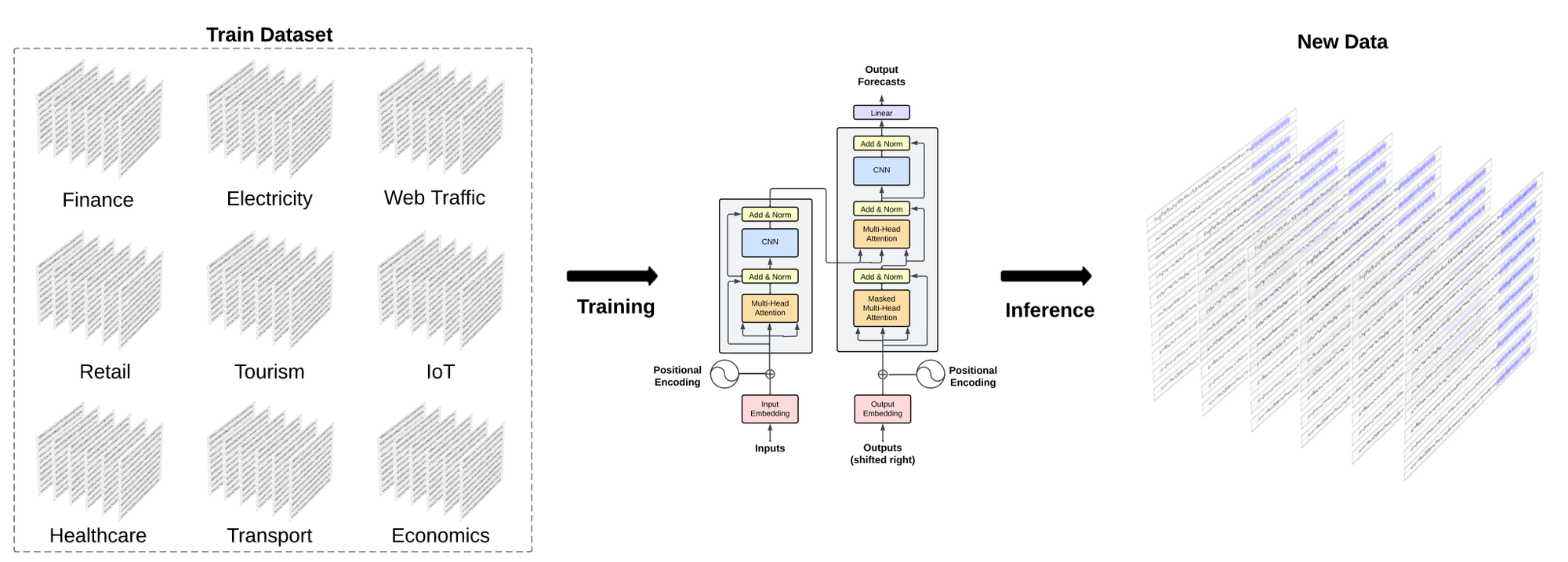 Figure 2: TimeGPT was trained on a collection of public datasets with different sizes and granularities to forecast unseen time series accurately without re-training (source).
Architecture
TimeGPT is a Transformer-based model specifically designed for time series forecasting, incorporating a self-attention mechanism within an encoder-decoder architecture. By leveraging the self-attention mechanism, it can dynamically weigh the significance of different points in the time series.
The model receives a window of historical values (y) and exogenous covariates (x) as input. The covariates may include additional time series data and/or binary variables that denote specific events, such as public holidays. These inputs are augmented with sequential information by integrating local positional embeddings. This allows the model to be aware of the temporal dependencies. While not explicitly stated by the authors, we believe all the inputs are concatenated after the positional encoding, producing the final input to feed the encoder.
 Figure 3: Process of adding positional embeddings to the input data and concatenating all inputs in a final input vector (image by author)
The positional encodings are also not defined by the authors. We assume that they use the sine and cosine functions from the foundational transformer architecture paper [7]. These functions are characterized by varying frequencies but maintain the same dimensionality as the input data.
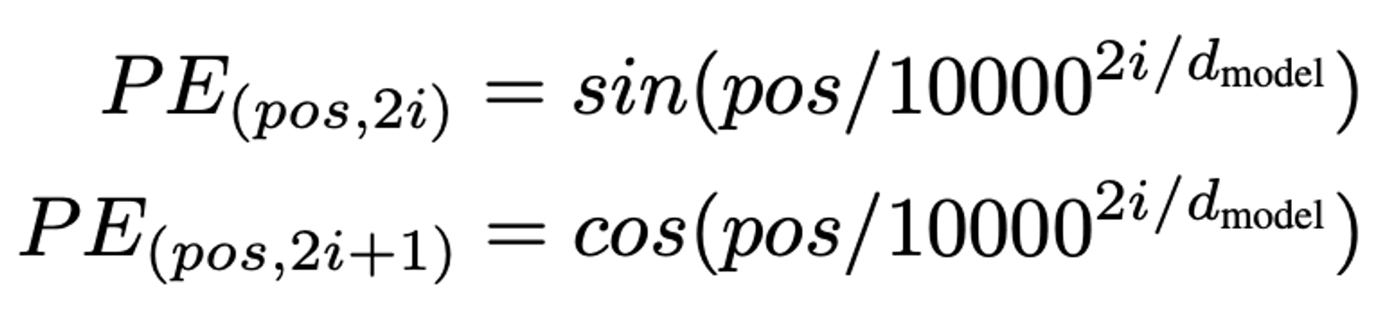 Equations 1: sine and cosine functions that generate positional embeddings where pos is the position, i is the dimension of the positional encoding, and _d model is the total dimension of the vector.
Once augmented with positional encodings, the input vector is introduced into the encoder. Within the encoder, a multi-head attention layer evaluates and assigns weights to the various elements within the input sequence, reflecting their relative importance. Subsequently, this representation is processed by a fully connected feed-forward network. It allows the generation of a representation that captures more complex relationships between the elements in the sequence. The output is then fed to the decoder part of the architecture.
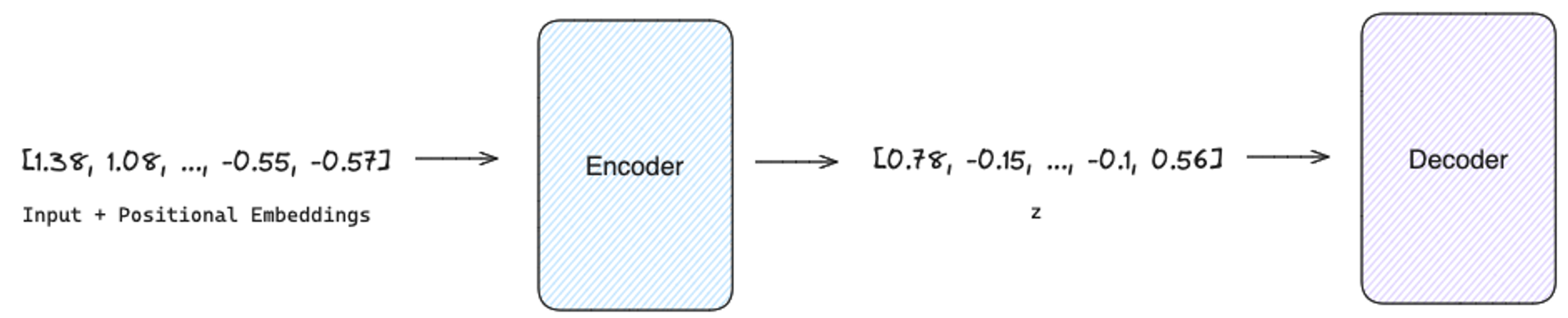 Figure 4: The Encoder receives the vector resulting from the addition between the input and the positional encoding and generates a new vector to feed the decoder (image by author)
In addition to processing the encoder's output, the decoder operates in an auto-regressive process. It incorporates previously generated outputs before producing the forecasts of the subsequent time step (i+1). It leverages the attention mechanism to capture the complex relationships between the hidden states produced by the encoder and the previously generated outputs. This approach enables the decoder to effectively synthesize the contextual and sequential information encapsulated in the encoder's representations with its own iterative predictions.
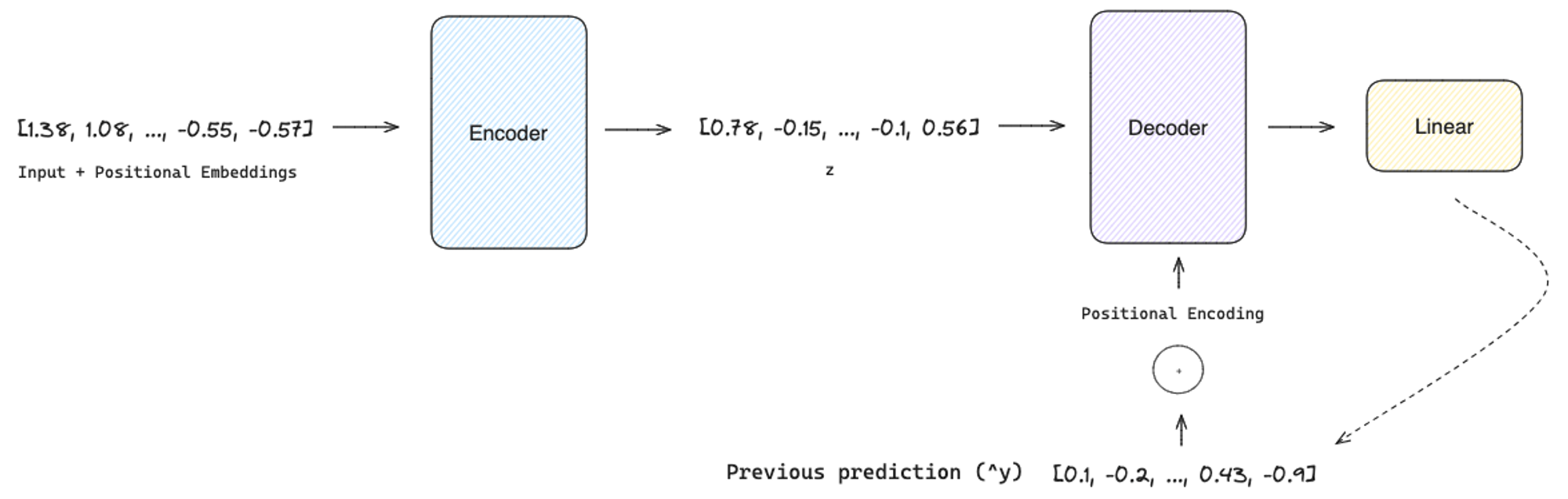 Figure 5: Decoder receives as input the output of the encoder and previous predictions position encoded (image by author)
Finally, the linear layer is responsible for mapping the decoder's output to a vector of values with the same length as the forecast horizon (h).
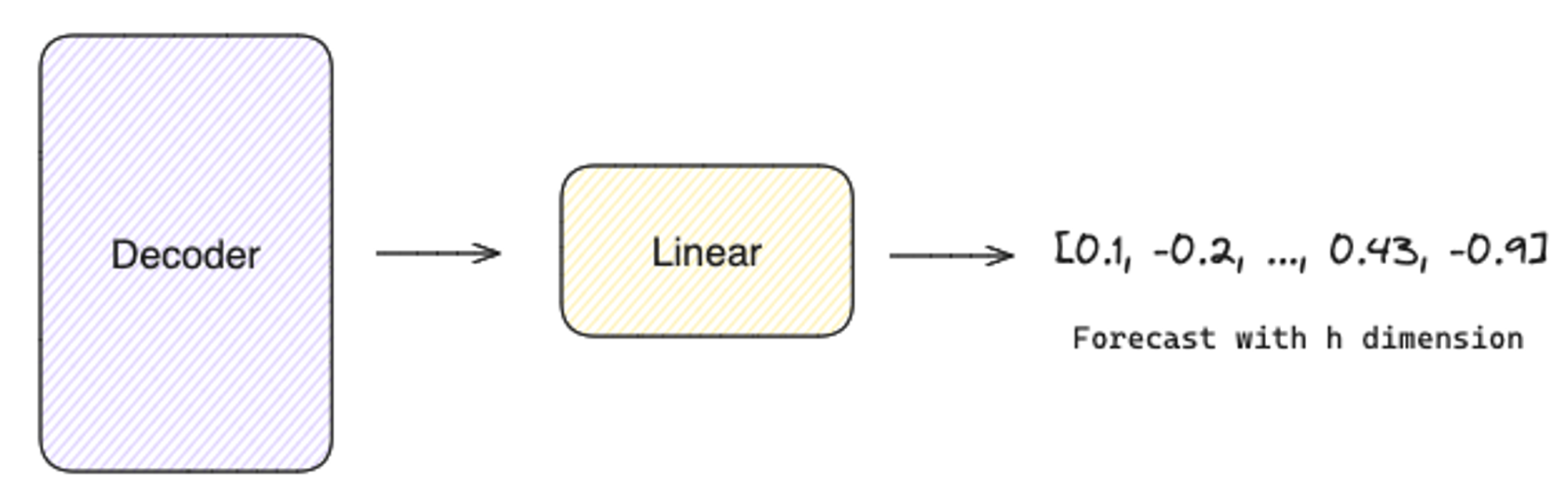 Figure 6: A linear layer receives the output of the decoder as input and produces the final forecast with the same dimension as the forecast horizon (image by author)
TimeGPT can generate a probabilistic distribution of potential outcomes, i.e., the estimation of forecast intervals. The authors relied on conformal prediction [8] based on historical errors to estimate the forecast intervals. Unlike traditional methods, conformal prediction does not require distributional assumptions, and it can be achieved by:
- Creating M training and calibration sets;
- Forecasting each calibration set with the model;
- For each forecast horizon h , the absolute residual values between the model's predictions and the actual outcomes within the calibration set are calculated. These calculated residuals are called nonconformity scores.
- We select a specific quantile from the distribution of nonconformity scores for each forecast horizon h. The chosen quantile determines the forecast interval's coverage level, with higher quantiles resulting in broader intervals.
The forecast intervals are given by the predicted value ± the final nonconformity score.
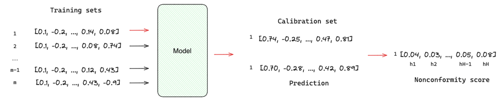 Figure 7: Conformal Prediction process (image by author)
TimeGPT vs. TiDE: a comparison in a real use case
In this section, we will use TimeGPT to forecast sales using a real-world dataset from one of our clients. Subsequently, we compare the forecasting performance of TimeGPT with TiDE, using the same cutoff date for analysis.
TiDE [2] is a novel multivariate time-series model that can use static covariates (e.g., brand of a product) and known or unknown dynamic covariates in the forecast horizon (e.g., price of a product) to generate an accurate forecast. Unlike the complex architecture of Transformers, TiDE is based on a simple Encoder-Decoder architecture with a Residual connection where:
- The Encoder is responsible for mapping the past target values and the covariates of a time series into a dense representation of features. First, the feature projection reduces the dimensionality of the dynamic covariates. Then, the Dense Encoder receives the output of the Feature Projection concatenated with static covariates and the past values to map them into a single embedding representation.
- The Decoder receives the embedding representation and converts it into future predictions. The Dense Decoder maps the embedding representation into a vector per time-step in the horizon. Afterward, the Temporal Decoder combines the output of the Dense Decoder with the projected features of that time step to produce the predictions.
- Finally, the Residual Connection linearly maps the look-back to a vector with the size of the horizon, which is added to the output of the Temporal Decoder to produce the final predictions.
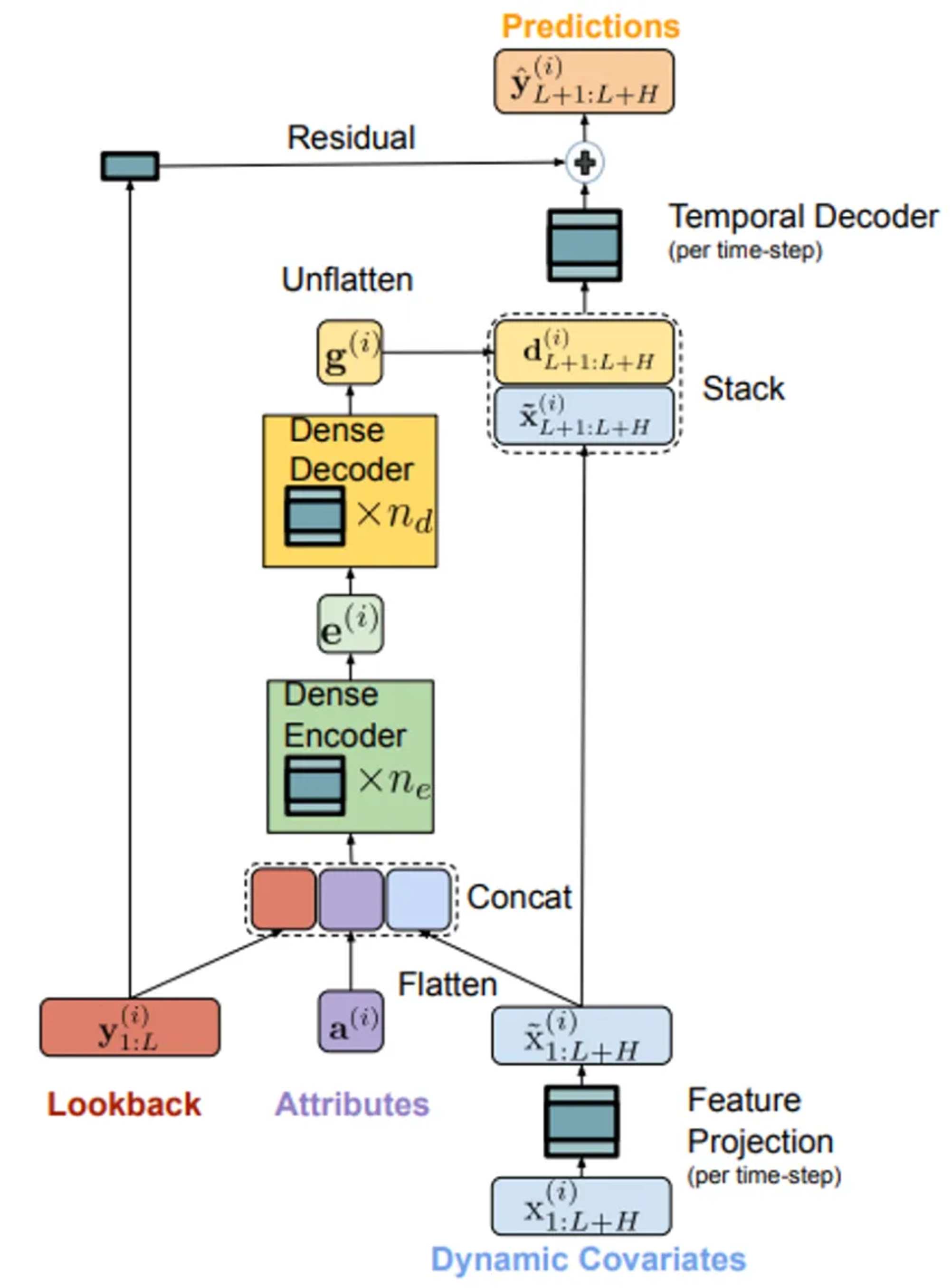 Figure 8: TiDE architecture (source)
The dataset contains 195 unique time series, each detailing weekly sales data specifically for the United States market. In addition to historical sales data, the dataset has information on two types of marketing events. We incorporate US public holidays and binary seasonal features to augment the dataset, in this case, week and month identifiers. The forecasting horizon is 16 weeks, i.e., we want to predict 16 weeks into the future.
We start by importing the libraries:
javascript
import matplotlib.pyplot as plt
import os
import pandas as pd
import utils

from nixtlats import TimeGPT
from nixtlats.date_features import CountryHolidays
from dotenv import load_dotenv
from sklearn.preprocessing import MinMaxScaler, OrdinalEncoder

load_dotenv()
Then, we initiate the TimeGPT class by providing a TimeGPT token. You can request one from the Nixtla website.
csharp
timegpt = TimeGPT(token = os.environ.get("TIMEGPT_KEY"))
timegpt.validate_token()
INFO:nixtlats.timegpt:Happy Forecasting! :), If you have questions or need support, please email ops@nixtla.io
When preparing to load your dataset after validating the authentication token, ensure the following:
- The target variable should be numeric and without missing values.
- Ensure no gaps exist in the date sequence from the start to the end date.
- The date column must be in a format recognizable by Pandas.
- Per the documentation, data normalization is handled internally. Therefore, you can skip that step.
- For forecasting multiple time series, include a column to uniquely identify each series, which will be used as an argument in the forecasting function.
- Exogenous features require a separate dataset for the forecast horizon.
ini
# read data frame and parse dates as datetime
df = pd.read_csv('data/data.csv', parse_dates=['delivery_week'])
As discussed, to augment the dataset, we add binary seasonal features for week and month as follows:
bash
# add week and month to df
df['week'] = df['delivery_week'].dt.isocalendar().week
df['month'] = df['delivery_week'].dt.month

# one hot encode week and month
df = pd.get_dummies(df, columns=['week', 'month'], dtype=int)
Now, we can truncate our dataset to be used by TimeGPT for forecasting. Additionally, we will create a holdout set with the actual sales data within the forecast horizon and the corresponding exogenous features for the same period.
bash
# Truncate data frame
forecast_df = df[df['delivery_week'] < "2023-10-16"]
# Let's use the last x weeks of actuals for the holdout set
holdout_df = df[(df['delivery_week'] >= "2023-10-16") & (df['delivery_week'] <= "2024-02-05")]
After splitting the data, we can proceed to feed the training and holdout datasets into the forecast() function. We need to set the following parameters:
df - data frame with historical datatime_col - column with temporal informationtarget_col - column with historical dataX_df - data frame with exogenous features for the forecast horizondate_features - allows the specification of new exogenous features like the public holidays in the USh - define the forecast horizonlevel - forecast intervals (80% confidence)freq - frequency of the data, in our case, it is weekly on Mondayid_col - column that identifies each time series in a multivariate scenariomodel - TimeGPT has two models one for short term and another for long term. The long-term should be used when there is more than one seasonal period in the forecast horizon.add_history - return the fitted values in historical data
bash
# create list with seasonal exogenous features
EXOGENOUS_FAETURES = [x for x in df.columns if ('week_' in x) | ('month_' in x)]

timegpt_fcst_ex_vars_df = timegpt.forecast(
    df=forecast_df[['unique_id', 'delivery_week', 'target', 'marketing_events_1', 'marketing_events_2']+EXOGENOUS_FAETURES],
    time_col='delivery_week',
    target_col='target',
    X_df=holdout_df[['unique_id', 'delivery_week', 'marketing_events_1', 'marketing_events_2']+EXOGENOUS_FAETURES],
    date_features=[CountryHolidays(['US'])],
    h=17,
    level=[80],
    freq='W-MON',
    id_col='unique_id',
    model='timegpt-1',
    add_history=True,
    )
The forecast takes just a few minutes to run. It then returns a data frame with the fitted values for historical data and the predictions for the forecast horizon. It also returns the importance of the exogenous covariates in the forecast.
csharp
timegpt.weights_x.head(10).sort_values(by='weights').plot.barh(x='features', y='weights')
plt.title('Feature Importance - top 10')
plt.show()
In our case, we extracted the ten most important covariates, which shows that the marketing events have the highest importance. Conversely, the seasonal and holidays covariates have a residual importance.
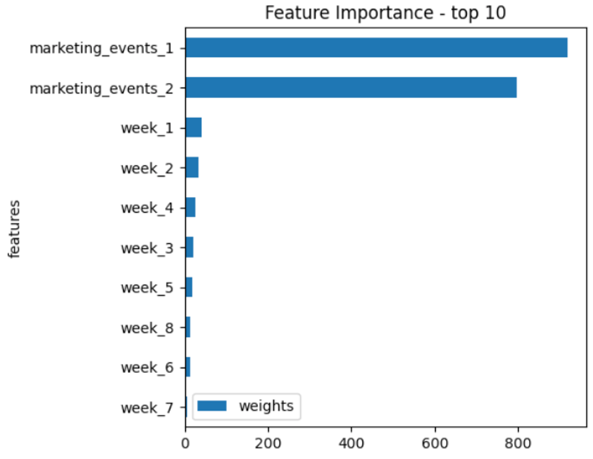 Figure 9: TimeGPT exogenous covariates importance (image made by the author)
Since we set
add_history=True, we can plot the fitted values and the predictions. We selected the six series with the highest volume in the holdout set. They are more relevant for the business and likely easier to forecast with more stable patterns.
python
# get series ordered by volume in a descending way
series = holdout_df.groupby('unique_id')['target'].sum().reset_index().sort_values(by='target', ascending=False)['unique_id'].tolist()

timegpt.plot(
    forecast_df[['unique_id', 'delivery_week', 'target']],
    timegpt_fcst_ex_vars_df,
    time_col='delivery_week',
    target_col='target',
    unique_ids=series[:6],
    level=[80],
)
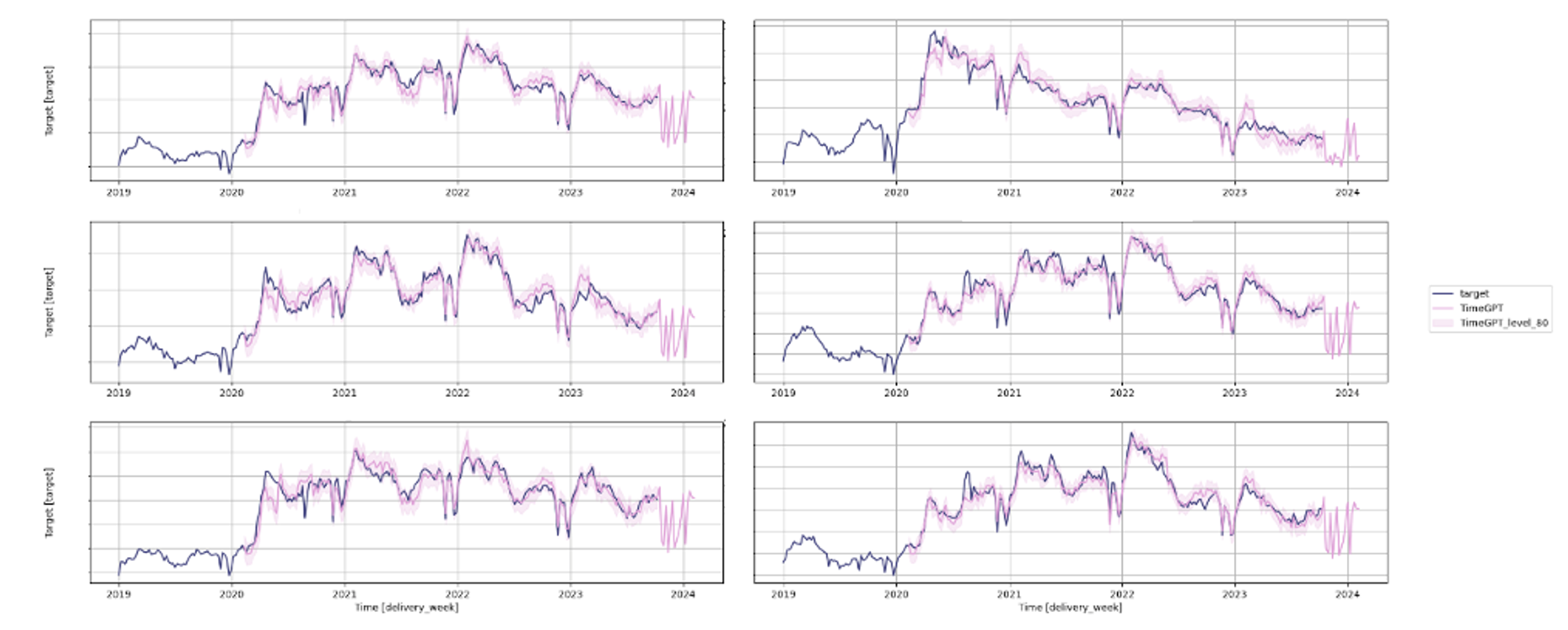 Figure 10: TimeGPT fitted values and forecast (image by author)
Figure 10 shows that while the fitted values align well with the actual values, the forecasts are inconsistent. They show uniform patterns across most series except in one case (we can find it in the top right corner). Additionally, all predictions show consecutive unexpected spikes, which we did not expect to see.
Having obtained the forecast from TimeGPT, we can now load the forecast generated by TiDE and compute forecasting performance metrics for comparison. We have used the Mean Absolute Percentage Error (MAPE) as our comparison metric to maintain confidentiality and prevent the disclosure of actual sales volumes.
python
# load the forecast from TiDE and TimeGPT
tide_model_df = pd.read_csv('data/tide.csv', parse_dates=['delivery_week'])
timegpt_fcst_ex_vars_df = pd.read_csv('data/timegpt.csv', parse_dates=['delivery_week'])

# merge data frames with TiDE forecast and actuals
model_eval_df = pd.merge(holdout_df[['unique_id', 'delivery_week', 'target']], tide_model_df[['unique_id', 'delivery_week', 'forecast']], on=['unique_id', 'delivery_week'], how='inner')

# merge data frames with TimeGPT forecast and actuals
model_eval_df = pd.merge(model_eval_df, timegpt_fcst_ex_vars_df[['unique_id', 'delivery_week', 'TimeGPT']], on=['unique_id', 'delivery_week'], how='inner')

utils.plot_model_comparison(model_eval_df)
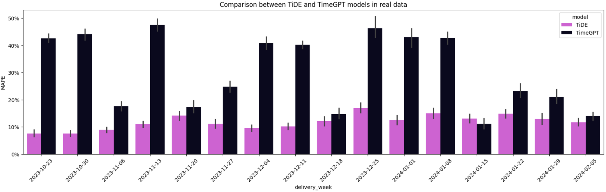 Figure 11: MAPE comparison between TiDE and TimeGPT (image by author)
As shown in Figure 11, TiDE has a lower average MAPE when compared to TimeGPT across the 195-time series for 15 out of 16 weeks. Although both models have access to the same information, the zero-shot inference from TimeGPT did not manage to beat our fine-tuned model.
Conclusion
The significance of forecasting cannot be overstated in today's competitive landscape. Effective forecasting methods are key for organizations striving for operational excellence, enabling them to plan and manage their operations more efficiently.
In this article, we explored one of the most recent innovations in time series forecasting - the development of foundation models. These models aim to democratize access to sophisticated algorithms for organizations lacking the specialized expertise required to develop SOTA models in-house. While this initiative is promising, our analysis indicates that it still falls short of delivering accurate forecasts. Specifically, TiDE significantly outperformed TimeGPT in a zero-shot inference scenario.
Nevertheless, it is encouraging to witness the efforts of AI companies to push the boundaries of forecasting. While other domains, such as computer vision and NLP, have been gaining increased attention, the significance of forecasting for organizations should not be overlooked.
About me
Serial entrepreneur and leader in the AI space. I develop AI products for businesses and invest in AI-focused startups.
Founder @ ZAAI | LinkedIn | X/Twitter
References
[1] Garza, A., & Mergenthaler-Canseco, M. (2023). TimeGPT-1. Retrieved from arXiv:2310.03589.
[2] Abhimanyu Das, Weihao Kong, Andrew Leach, Shaan Mathur, Rajat Sen, Rose Yu. (2023) Long-term Forecasting with TiDE: Time-series Dense Encoder. arXiv:2304.08424.
[3] Goswami, M., Szafer, K., Choudhry, A., Cai, Y., Li, S., & Dubrawski, A. (2024). MOMENT: A Family of Open Time-series Foundation Models. Retrieved from arXiv:2402.03885 (cs.LG).
[4] Das, A., Kong, W., Sen, R., & Zhou, Y. (2024). A decoder-only foundation model for time-series forecasting. Retrieved from arXiv:2310.10688 (cs.CL).
[5] Rasul, K., Ashok, A., Williams, A. R., Ghonia, H., Bhagwatkar, R., Khorasani, A., Darvishi Bayazi, M. J., Adamopoulos, G., Riachi, R., Hassen, N., Biloš, M., Garg, S., Schneider, A., Chapados, N., Drouin, A., Zantedeschi, V., Nevmyvaka, Y., & Rish, I. (2024). Lag-Llama: Towards Foundation Models for Probabilistic Time Series Forecasting. Retrieved from arXiv:2310.08278 (cs.LG).
[6] Woo, G., Liu, C., Kumar, A., Xiong, C., Savarese, S., & Sahoo, D. (2024). Unified Training of Universal Time Series Forecasting Transformers. Retrieved from arXiv:2402.02592 (cs.LG).
[7] Vaswani, A., Shazeer, N., Parmar, N., Uszkoreit, J., Jones, L., Gomez, A. N., Kaiser, L., & Polosukhin, I. (2017). Attention Is All You Need. Retrieved from arXiv:1706.03762.
[8] Stankeviciute, K., Alaa, A. M., & van der Schaar, M. (2021). Conformal time-series forecasting. In Advances in Neural Information Processing Systems (Vol. 34, pp. 6216–6228).
Register Now to Continue Reading
Unlock Towards Data Science with a Free Account
All articles on Towards Data Science are available to registered users. Create a free account today to access this article and thousands more.
Register for freeSign in to your account
 Written By
See all from Luís Roque
Artificial IntelligenceData ScienceMachine LearningPythonTime Series Forecasting
Share This Article
Towards Data Science is a community publication. Submit your insights to reach our global audience and earn through the TDS Author Payment Program.
Write for TDS
Related Articles
Data Science
Analyzing the Italian Soccer League (The Serie A as it's known) reveals a lot about how sport changes quickly
Azaan Barlas
November 17, 20218 min read
Data Science
Everything you wanted to know about it and its main actors
Victor Roman
September 27, 20197 min read
Data Science
My experience from interviewing as a Data Scientist in 2021 in Bangalore, India.
Divya Choudhary
July 5, 20215 min read
Data Science
A supply chain network footprint should include greenhouse gas calculations for both transportation and distribution centers
Sabi Horvat
April 25, 20235 min read
Data Science
People are the most critical part of businesses. People create value for people and sell it to people. Therefore, changes on people and...
Soner Yıldırım
January 5, 202012 min read
Data Science
Quick tips and examples to create data visualizations using the Bokeh library
Payal Patel
December 16, 202211 min read
Machine Learning
Removing unwanted sub-strings from a column in Pandas
Giorgos Myrianthous
March 29, 20225 min read
Data Science
The potential of data analytics is often held back by ancient and diverse legacy system scattered across the company. However, data and...
Wouter van Heeswijk, PhD
October 10, 20217 min read
Data Science
A stance on the opportunity for out-of-the-box insight for standard schemas
Charles Zhu
October 23, 202011 min read
Your home for data science and AI. The world's leading publication for data science, data analytics, data engineering, machine learning, and artificial intelligence professionals.
Subscribe to Our NewsletterWrite For TDS•About•Advertise•Privacy Policy•Terms of Use
© Insight Media Group, LLC 2026•The New Stack•roadmap.sh•Creator Network