保留正文与补采附件。源页面当前未重新核验;具体限制见交付清单。
 We value your privacy
We use cookies to enhance your browsing experience, serve personalised ads or content, and analyse our traffic. By clicking "Accept All", you consent to our use of cookies.
Customise Reject All Accept All
Customise Consent Preferences
 We use cookies to help you navigate efficiently and perform certain functions. You will find detailed information about all cookies under each consent category below.
The cookies that are categorised as "Necessary" are stored on your browser as they are essential for enabling the basic functionalities of the site. ... Show more
NecessaryAlways Active
Necessary cookies are required to enable the basic features of this site, such as providing secure log-in or adjusting your consent preferences. These cookies do not store any personally identifiable data.
-
Cookie
BCTempID
-
Duration
10 minutes
-
Description
No description available.
-
Cookie
__cf_bm
-
Duration
1 hour
-
Description
This cookie, set by Cloudflare, is used to support Cloudflare Bot Management.
-
Cookie
AWSALBCORS
-
Duration
7 days
-
Description
Amazon Web Services set this cookie for load balancing.
-
Cookie
_cfuvid
-
Duration
session
-
Description
Cloudflare sets this cookie to track users across sessions to optimize user experience by maintaining session consistency and providing personalized services
-
Cookie
li_gc
-
Duration
6 months
-
Description
Linkedin set this cookie for storing visitor's consent regarding using cookies for non-essential purposes.
-
Cookie
__hssrc
-
Duration
session
-
Description
This cookie is set by Hubspot whenever it changes the session cookie. The __hssrc cookie set to 1 indicates that the user has restarted the browser, and if the cookie does not exist, it is assumed to be a new session.
-
Cookie
__hssc
-
Duration
1 hour
-
Description
HubSpot sets this cookie to keep track of sessions and to determine if HubSpot should increment the session number and timestamps in the __hstc cookie.
-
Cookie
wpEmojiSettingsSupports
-
Duration
session
-
Description
WordPress sets this cookie when a user interacts with emojis on a WordPress site. It helps determine if the user's browser can display emojis properly.
-
Cookie
BCSessionID
-
Duration
1 year 1 month 4 days
-
Description
Blueconic sets this cookie as a unique identifier for the BlueConic profile.
-
Cookie
_octo
-
Duration
1 year
-
Description
No description available.
-
Cookie
logged_in
-
Duration
1 year
-
Description
No description available.
-
Cookie
__Secure-YEC
-
Duration
past
-
Description
YouTube sets this cookie to stores the user's video player preferences using embedded YouTube video
-
Cookie
__eoi
-
Duration
6 months
-
Description
Description is currently not available.
-
Cookie
AWSALBTGCORS
-
Duration
7 days
-
Description
No description available.
-
Cookie
login-status-p
-
Duration
past
-
Description
Description is currently not available.
-
Cookie
AWSALBTG
-
Duration
7 days
-
Description
No description available.
-
Cookie
csrf_token
-
Duration
session
-
Description
No description available.
-
Cookie
token_v2
-
Duration
1 day
-
Description
Description is currently not available.
-
Cookie
D
-
Duration
1 year
-
Description
Description is currently not available.
-
Cookie
PHPSESSID
-
Duration
session
-
Description
This cookie is native to PHP applications. The cookie stores and identifies a user's unique session ID to manage user sessions on the website. The cookie is a session cookie and will be deleted when all the browser windows are closed.
-
Cookie
VISITOR_PRIVACY_METADATA
-
Duration
6 months
-
Description
YouTube sets this cookie to store the user's cookie consent state for the current domain.
-
Cookie
cookietest
-
Duration
session
-
Description
The cookietest cookie is typically used to determine whether the user's browser accepts cookies, essential for website functionality and user experience.
-
Cookie
__Host-airtable-session
-
Duration
1 year
-
Description
This cookie is used to enable us to integrate the services of Airtable.
-
Cookie
__Host-airtable-session.sig
-
Duration
1 year
-
Description
This cookie is used to enable us to integrate the services of Airtable.
-
Cookie
m
-
Duration
1 year 1 month 4 days
-
Description
Stripe sets this cookie for fraud prevention purposes. It identifies the device used to access the website, allowing the website to be formatted accordingly.
-
Cookie
BIGipServer*
-
Duration
session
-
Description
Marketo sets this cookie to collect information about the user's online activity and build a profile about their interests to provide advertisements relevant to the user.
-
Cookie
__cfruid
-
Duration
session
-
Description
Cloudflare sets this cookie to identify trusted web traffic.
-
Cookie
_GRECAPTCHA
-
Duration
6 months
-
Description
Google Recaptcha service sets this cookie to identify bots to protect the website against malicious spam attacks.
-
Cookie
__Secure-YNID
-
Duration
6 months
-
Description
Google cookie used to protect user security and prevent fraud, especially during the login process.
-
Cookie
cookieyes-consent
-
Duration
1 year
-
Description
CookieYes sets this cookie to remember users' consent preferences so that their preferences are respected on subsequent visits to this site. It does not collect or store any personal information about the site visitors.
Functional
Functional cookies help perform certain functionalities like sharing the content of the website on social media platforms, collecting feedback, and other third-party features.
-
Cookie
lidc
-
Duration
1 day
-
Description
LinkedIn sets the lidc cookie to facilitate data center selection.
-
Cookie
brw
-
Duration
1 year
-
Description
No description available.
-
Cookie
brwConsent
-
Duration
5 minutes
-
Description
Description is currently not available.
-
Cookie
WMF-Uniq
-
Duration
1 year
-
Description
Description is currently not available.
-
Cookie
loom_anon_comment
-
Duration
1 year
-
Description
No description available.
-
Cookie
loom_referral_video
-
Duration
session
-
Description
Description is currently not available.
-
Cookie
VISITOR_INFO1_LIVE
-
Duration
6 months
-
Description
A cookie set by YouTube to measure bandwidth that determines whether the user gets the new or old player interface.
-
Cookie
yt-remote-connected-devices
-
Duration
Never Expires
-
Description
YouTube sets this cookie to store the user's video preferences using embedded YouTube videos.
-
Cookie
ytidb::LAST_RESULT_ENTRY_KEY
-
Duration
Never Expires
-
Description
The cookie ytidb::LAST_RESULT_ENTRY_KEY is used by YouTube to store the last search result entry that was clicked by the user. This information is used to improve the user experience by providing more relevant search results in the future.
-
Cookie
yt-remote-device-id
-
Duration
Never Expires
-
Description
YouTube sets this cookie to store the user's video preferences using embedded YouTube videos.
-
Cookie
yt-remote-session-name
-
Duration
session
-
Description
The yt-remote-session-name cookie is used by YouTube to store the user's video player preferences using embedded YouTube video.
-
Cookie
yt-remote-fast-check-period
-
Duration
session
-
Description
The yt-remote-fast-check-period cookie is used by YouTube to store the user's video player preferences for embedded YouTube videos.
-
Cookie
yt-remote-session-app
-
Duration
session
-
Description
The yt-remote-session-app cookie is used by YouTube to store user preferences and information about the interface of the embedded YouTube video player.
-
Cookie
yt-remote-cast-available
-
Duration
session
-
Description
The yt-remote-cast-available cookie is used to store the user's preferences regarding whether casting is available on their YouTube video player.
-
Cookie
yt-remote-cast-installed
-
Duration
session
-
Description
The yt-remote-cast-installed cookie is used to store the user's video player preferences using embedded YouTube video.
-
Cookie
cp_session
-
Duration
3 months
-
Description
Codepen sets this cookie for Help systems found in the website.
-
Cookie
loid
-
Duration
1 year 1 month 4 days
-
Description
This cookie is set by the Reddit. The cookie enables the sharing of content from the website onto the social media platform.
Analytics
Analytical cookies are used to understand how visitors interact with the website. These cookies help provide information on metrics such as the number of visitors, bounce rate, traffic source, etc.
-
Cookie
__hstc
-
Duration
6 months
-
Description
Hubspot set this main cookie for tracking visitors. It contains the domain, initial timestamp (first visit), last timestamp (last visit), current timestamp (this visit), and session number (increments for each subsequent session).
-
Cookie
hubspotutk
-
Duration
6 months
-
Description
HubSpot sets this cookie to keep track of the visitors to the website. This cookie is passed to HubSpot on form submission and used when deduplicating contacts.
-
Cookie
_ga
-
Duration
1 year 1 month 4 days
-
Description
Google Analytics sets this cookie to calculate visitor, session and campaign data and track site usage for the site's analytics report. The cookie stores information anonymously and assigns a randomly generated number to recognise unique visitors.
-
Cookie
ga*
-
Duration
1 year 1 month 4 days
-
Description
Google Analytics sets this cookie to store and count page views.
-
Cookie
__Host-psifi.analyticsTrace
-
Duration
6 hours
-
Description
Description is currently not available.
-
Cookie
__Host-psifi.analyticsTraceV2
-
Duration
6 hours
-
Description
Description is currently not available.
-
Cookie
_gh_sess
-
Duration
session
-
Description
GitHub sets this cookie for temporary application and framework state between pages like what step the user is on in a multiple step form.
-
Cookie
YSC
-
Duration
session
-
Description
YSC cookie is set by Youtube and is used to track the views of embedded videos on Youtube pages.
-
Cookie
ajs_anonymous_id
-
Duration
1 year
-
Description
This cookie is set by Segment to count the number of people who visit a certain site by tracking if they have visited before.
-
Cookie
vuid
-
Duration
1 year 1 month 4 days
-
Description
Vimeo installs this cookie to collect tracking information by setting a unique ID to embed videos on the website.
Performance
Performance cookies are used to understand and analyse the key performance indexes of the website which helps in delivering a better user experience for the visitors.
-
Cookie
AWSALB
-
Duration
7 days
-
Description
AWSALB is an application load balancer cookie set by Amazon Web Services to map the session to the target.
-
Cookie
acq
-
Duration
past
-
Description
Description is currently not available.
-
Cookie
acq.sig
-
Duration
past
-
Description
Description is currently not available.
-
Cookie
ptc
-
Duration
2 years
-
Description
No description available.
Advertisement
Advertisement cookies are used to provide visitors with customised advertisements based on the pages you visited previously and to analyse the effectiveness of the ad campaigns.
-
Cookie
muc_ads
-
Duration
1 year 1 month 4 days
-
Description
Twitter sets this cookie to collect user behaviour and interaction data to optimize the website.
-
Cookie
guest_id_marketing
-
Duration
1 year 1 month 4 days
-
Description
Twitter sets this cookie to identify and track the website visitor.
-
Cookie
guest_id_ads
-
Duration
1 year 1 month 4 days
-
Description
Twitter sets this cookie to identify and track the website visitor.
-
Cookie
personalization_id
-
Duration
1 year 1 month 4 days
-
Description
Twitter sets this cookie to integrate and share features for social media and also store information about how the user uses the website, for tracking and targeting.
-
Cookie
guest_id
-
Duration
1 year 1 month 4 days
-
Description
Twitter sets this cookie to identify and track the website visitor. It registers if a user is signed in to the Twitter platform and collects information about ad preferences.
-
Cookie
bcookie
-
Duration
1 year
-
Description
LinkedIn sets this cookie from LinkedIn share buttons and ad tags to recognize browser IDs.
-
Cookie
__Secure-ROLLOUT_TOKEN
-
Duration
6 months
-
Description
YouTube sets this cookie to manage feature rollout and experimentation. It helps Google control which new features or interface changes are shown to users as part of testing and staged rollouts, ensuring consistent experience for a given user during an experiment.
-
Cookie
yt.innertube::nextId
-
Duration
Never Expires
-
Description
YouTube sets this cookie to register a unique ID to store data on what videos from YouTube the user has seen.
-
Cookie
yt.innertube::requests
-
Duration
Never Expires
-
Description
YouTube sets this cookie to register a unique ID to store data on what videos from YouTube the user has seen.
-
Cookie
session_tracker
-
Duration
session
-
Description
This cookie is set by the Reddit. This cookie is used to identify trusted web traffic. It also helps in adverstising on the website.
-
Cookie
edgebucket
-
Duration
session
-
Description
Reddit sets this cookie to save the information about a log-on Reddit user, for the purpose of advertisement recommendations and updating the content.
-
Cookie
did
-
Duration
1 year
-
Description
Arbor sets this cookie to show targeted ads to site visitors.This cookie expires after 2 months or 1 year.
Uncategorised
Other uncategorised cookies are those that are being analysed and have not been classified into a category as yet.
No cookies to display.
Reject All Save My Preferences Accept All
Toggle SearchToggle Mobile Navigation
Publish AI, ML & data-science insights to a global community of data professionals.
Sign inSubmit an Article
LatestEditor's PicksNewsletterShipAI
Write For TDS
LinkedInXToggle Search
Deep Learning
Towards Mamba State Space Models for Images, Videos and Time Series
Part 1
Sascha Kirch
August 14, 202417 min read
Towards Mamba State Space Models for Images, Videos and Time Series
 Image by Sascha Kirch
This is part 1 of my new multi-part series 🐍 Towards Mamba State Space Models for Images, Videos and Time Series.
Is Mamba all you need? Certainly, people have thought that for a long time of the Transformer architecture introduced by A. Vaswani et. al. in Attention is all you need back in 2017. And without any doubt, the transformer has revolutionized the field of deep learning over and over again. Its general-purpose architecture can easily be adapted for various data modalities such as text, images, videos and time series and it seems that the more compute resources and data you throw at the Transformer, the more performant it becomes.
However, the Transformer's attention mechanism has a major drawback: it is of complexity O(N²) , meaning it scales quadratically with the sequence length. This implies the larger the input sequence, the more compute resources you need, making large sequences often unfeasible to work with.
❓ The question is: can we do better? Is there a way we can reduce the O(N²) complexity while still being performant? And what would this new architecture look like?
🏊 ♂️ Jump in and join me in this multi-part deep dive series on Mamba state space models where we will discover why Mamba is an interesting new general-purpose approach for many applications and data modalities.
Outline
- What is this Series About?
- Why Do We Need a New Model?
- Structured State Space Models
- Here Comes Mamba
- Vision Mamba - Mamba Applied on Images
- VideoMamba - Understanding Videos
- MambaMixer - Adding Selectivity to Channels
- Mamba-2 - Closing the Gap Between Attention and SSMs
- Conclusion
- Further Readings & Resources
1. What is this series about?
Obviously, it is all about Mamba, the model to be said to replace the mighty Transformer! But how does it work? What are the details not mentioned in the papers? And how do you deal with all different kinds of data modalities? To these and more questions you will find answers in this series of articles.
Explicitly, in part 1 , we will kick off this series by understanding the strengths and weaknesses of RNNs and Transformers to motivate the need for a new architecture. Further, I'll provide a primer on all the upcoming parts of this series introducing many recent research papers that build upon the success of Mamba.
In part 2 we will look into structured state space models (SSMs) that provided the foundation for Mamba. We'll discover that while they solve the issue of the O(N²) complexity, other obstacles emerge like how to deal with long-range dependencies and how to increase their performance. We continue in part 3 with the introduction of Mamba and see how it forms a new general-purpose architecture that is trained fast, inferred fast and has a similar, and in some applications even superior, performance as the mighty Transformer.
Further down the road , we will dive into recent research papers like Vision Mamba, VideoMamba, MambaMixer and Mamba-2 to see how Mamba is extended to various data modalities such as images, videos and time signals and how it is constantly improved.
Mamba State Space Models for Images, Videos and Time Series
2. Why Do We Need a New Model?
To understand the need for a new model architecture, let's have a quick look on the two most prominent sequence models we had until recently: The Transformer and the Recurent Neuronal Network (RNN):
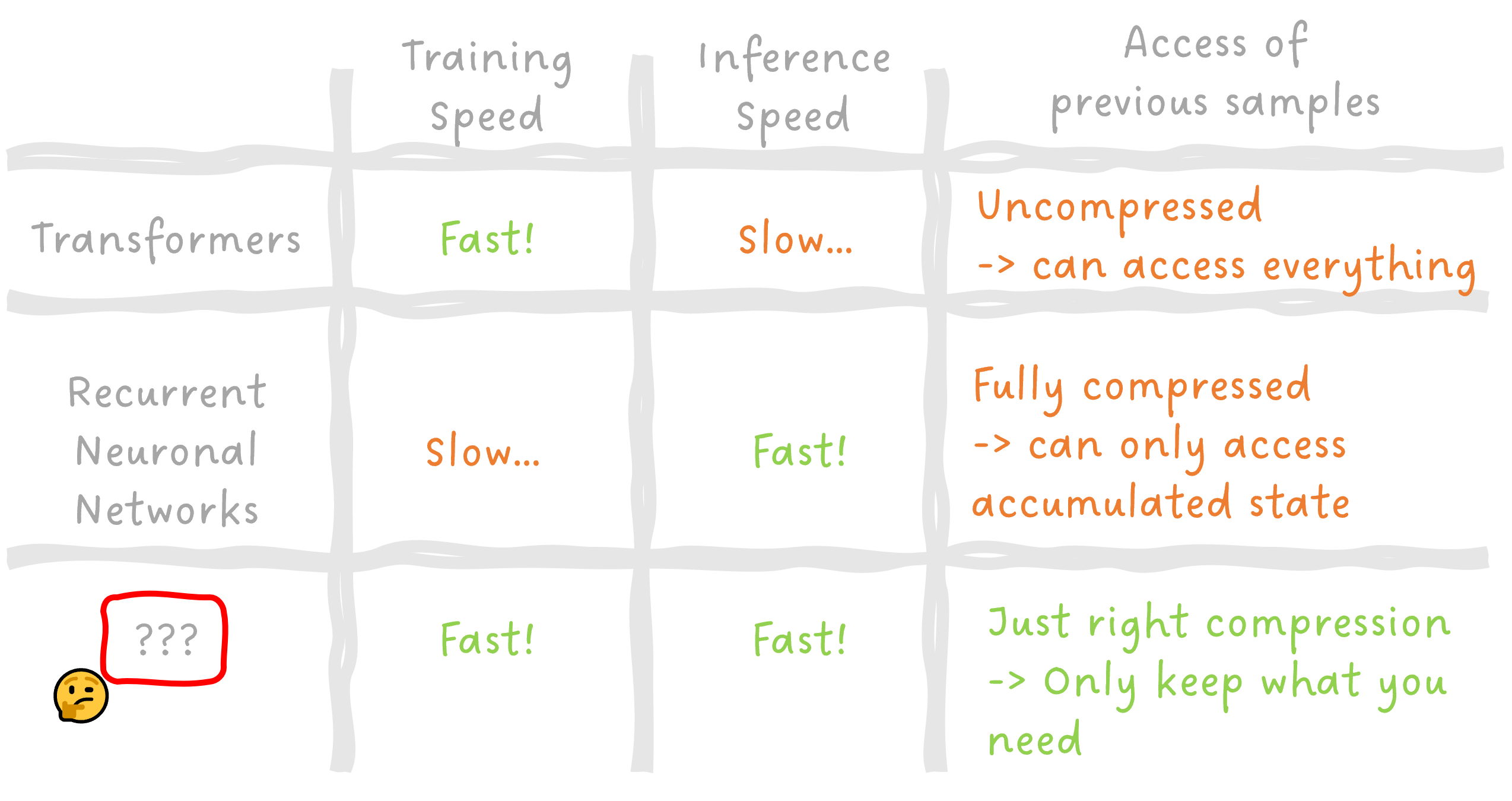 Image 1: Properties of Transformers, RNNs and the new model architecture we desire to find. Image by Sascha Kirch.
Ultimately, our goal is to have a model that trains fast, infers fast, while having a small memory footprint and does have access to all the relevant data of other samples of the sequence (Not more and not less).
Let's compare the RNN and the Transformer on a very high level:
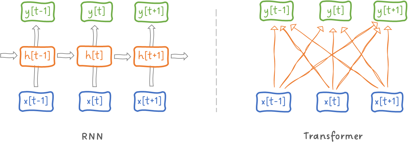 Image 2: Comparison of the high-level abstraction of how RNNs work vs. how Transformers work. Image by Sascha Kirch.
2.1 A Closer Look onto the RNN
In an RNN, the input x is propagated through the hidden state h to obtain the output y. Note that the output y[t] depends only on the hidden state h[t] and the current input x[t] and further note the current hidden state h[t] depends on the previous hidden state h[t-1] and the current input x[t]. This has the following implications:
- Past input samples can only be accessed through the hidden state that compresses the information of past data points and that must be updated for each new sample using the new input.
- We can only access samples from the past.
- Regardless of the length of the input, the number of computations per output stay constant and the total number of computations scale linearly with the length of the input sequence.
RNNs are fast at inference due to 3 , but cannot be parallelized during training due to 1 and 2. Especially the high compression of the state might limit the performance of the RNN compared to the Transformer. Due to the compression, valuable information might be lost especially when considering long sequences and the fact that the states need to be trained with a gradient based algorithm which might lead to difficulties like vanishing gradients.
2.2 What About the Transformer?
In the Transformer, each sample in the input sequence directly attends to itself and to every other sample of the sequence. In a sequence of N samples, each individual sample calculates a score on how much it attends to the other samples, which is the reason for the O(N²) complexity. This means that (for the vanilla attention mechanism):
- There is no compression at all between different samples and the state has a size of NxN.
- each sample can attend to previous and to future samples at once.
- If we do autoregressive sampling (e.g. next word prediction), we need to recompute all attention maps again to consider the new sample.
Especially 2 is the reason we can parallelize the Transformer well during training and it is 1 that its prediction performance is so good. You can tackle almost every problem with this brute force approach of letting everything attend to everything and let the Transformer figure out what it should look at to improve its performance. Since there is no compression, it is not hard to imagine that we also waste a lot of resources computing things that are irrelevant.
❓ The question is how do we get the best of both worlds? Fast training, fast sampling and efficiency in terms of memory.
🤔Might Mamba be a candidate to achieve exactly this?
3. Structured State Space Models
A primer for part 2 of this series
Let's start with the basics. Mamba builds on top of the idea of using state space models for deep learning. A state space model, as well known in system theory, describes the relationship between an input signal propagating through a stateful system and the resulting output signal.
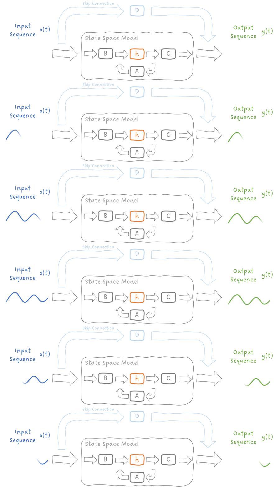 Image 3: Block diagram of a continuous-time state space model. Image by Sascha Kirch.
Since on a computer we work with discrete data, we need to discretize the state space model. Having the discrete state space model, we can uncover the two different representations: the recurrent representation and the convolutional representation. These two representations are equal, since the standard SSM is a linear and time-invariant (LTI) system.
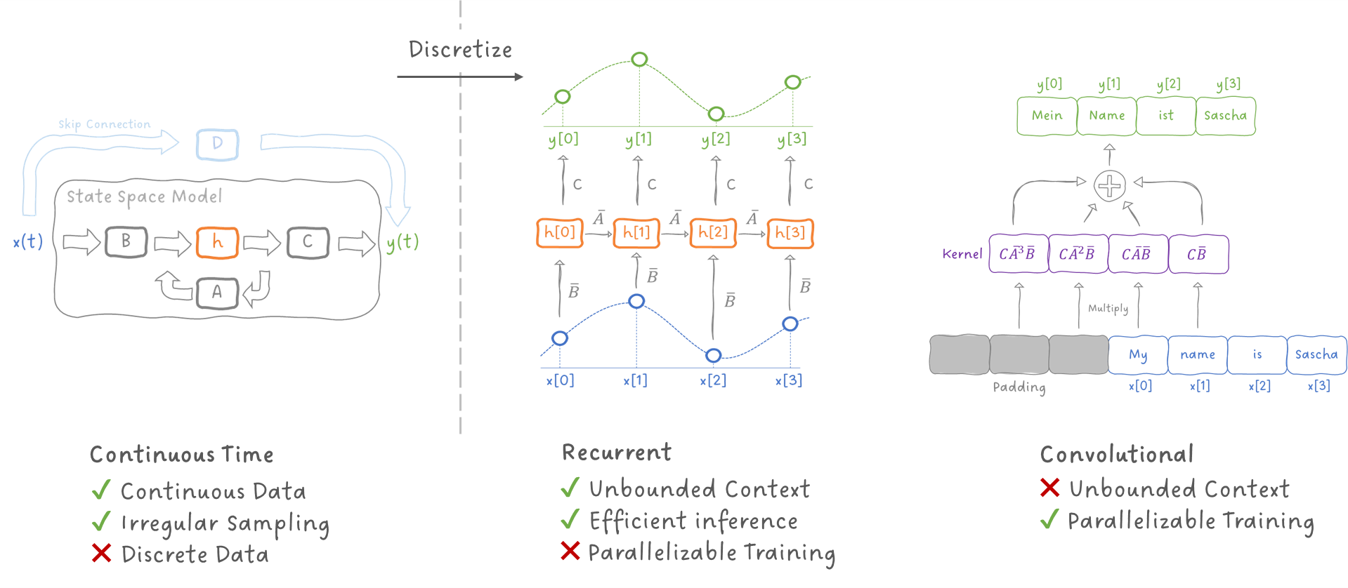 Image 4: Different representations of state space models. Image by Sascha Kirch.
We can leverage this duality and can use the recurrent representation for inference and the convolutional representation for training. This means the inference time scales linearly with the sequence length while we can train the model efficiently on modern hardware accelerators.
👉 What you'll find in part 2:
We will dive deeper into the formulation of the state space model and the state equations. We'll continue with the discretization and uncover the different representations of the SSM. We then change gears and discover how we resolve long range dependencies using the HiPPO framework and finally, we reach the S4 model, the structured state space sequence model, a milestone on the way towards Mamba. We will also discuss why we even care about structure in the involved matrices.
Structured State Space Models Visually Explained
4. Here Comes Mamba
A primer for part 3 of this series
With the S4 (Structured State Space Sequence Model) we ended up having a trainable state space model whose inference time scales linearly with the length of the input sequence and that can be trained efficiently leveraging the convolutional representation. Not only that, it also showed superior performance compared to the mighty Transformer (at least in the presented experiments).
The fact that S4 is a linear system, which we leveraged to switch between representations, is also its biggest weakness. Each sample of the input is treated equally because the matrices are time invariant. This is a big limitation because we might like to treat important inputs differently or probably ignore irrelevant inputs.
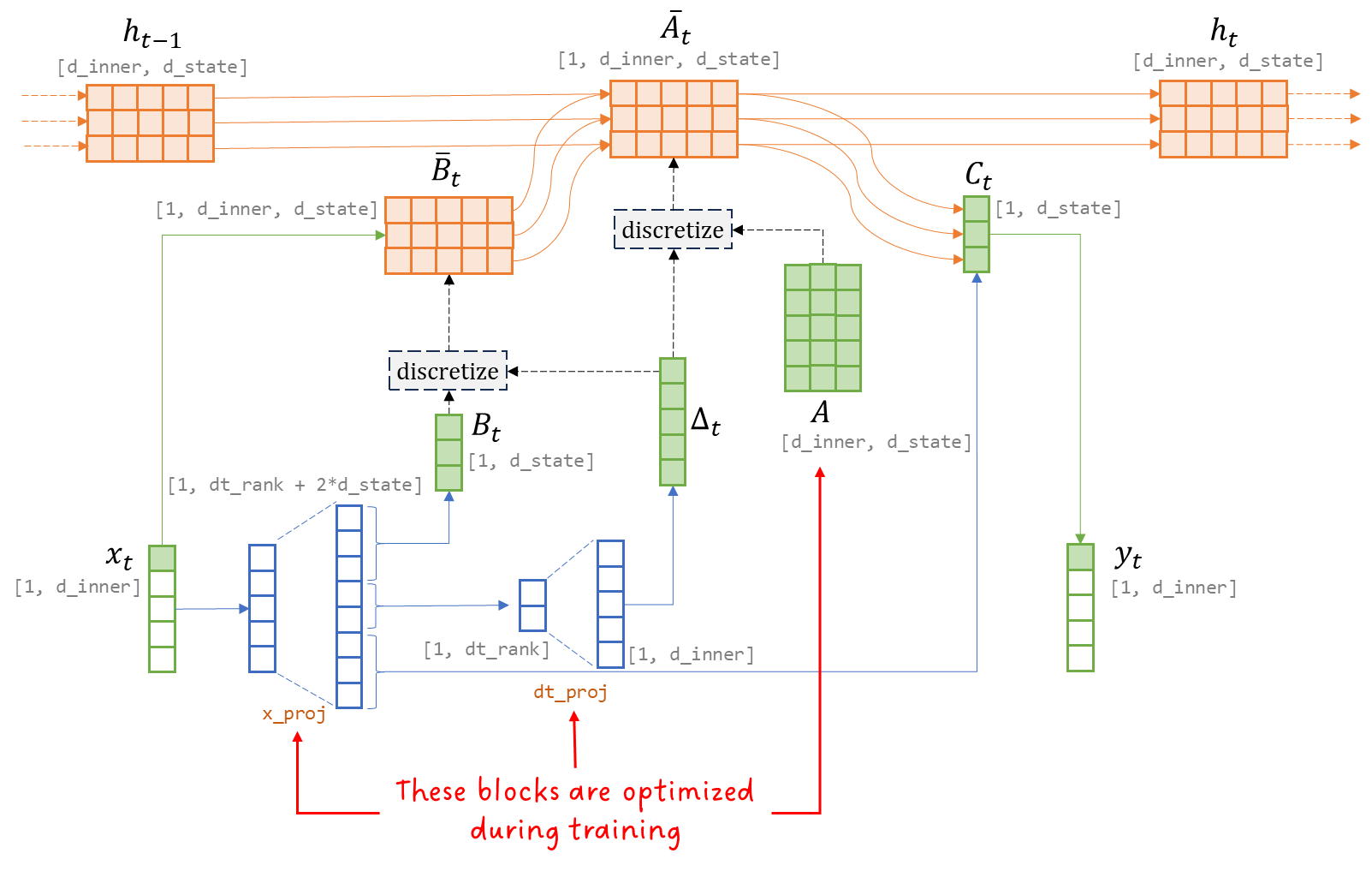 Image 5: Detailed view on the matrices involved in the selective state space model. Image by Sascha Kirch.
Mamba does exactly that: it makes the involved matrices time-variant to introduce the selectivity we want. As a consequence, we now have a time-varying system and we cannot use the convolutional representation anymore, hence we lose the possibility for fast and efficient training.
Mamba tackles this issue by further introducing a selective parallel scan, a technique combining kernel fusion, parallel associative scans and gradient recomputation to speed up the training of the model.
It further presents a general architecture, the Mamba Block, that just like the Transformer block can be stacked on top of each other build deep networks.
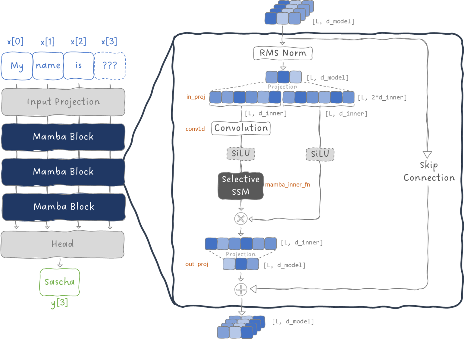 Image 6: Detailed block diagram of the Mamba-Block. Image by Sascha Kirch.
👉 What you will find in part 3:
We will talk about the selection mechanism of Mamba and see how this impacts the dimension of the involved matrices. We will further dive into the selective parallel scan and uncover what is behind the kernel fusion, the parallel associative scan and the recomputation of the gradients. Further, we will learn about the Mamba Block and I'll show you where the actually trained weights of the model hide and which dimensions they have (something that took me quite a while to understand to be honest)
Here Comes Mamba: The Selective State Space Model
Get an email whenever Sascha Kirch publishes 🚀 _Get an email whenever Sascha Kirch publishes 🚀 Looking to learn more about deep learning or simply stay up to dat_e...medium.com
5. Vision Mamba - Mamba Applied on Images
A primer for part 4 of this series
Having a new general architecture for sequence modeling, the Mamba Block, history starts to repeat itself. Just like the Transformer was applied to images by the introduction of the Vision Transformer (ViT), Mamba is applied to images resulting in Vision Mamba (Vim).
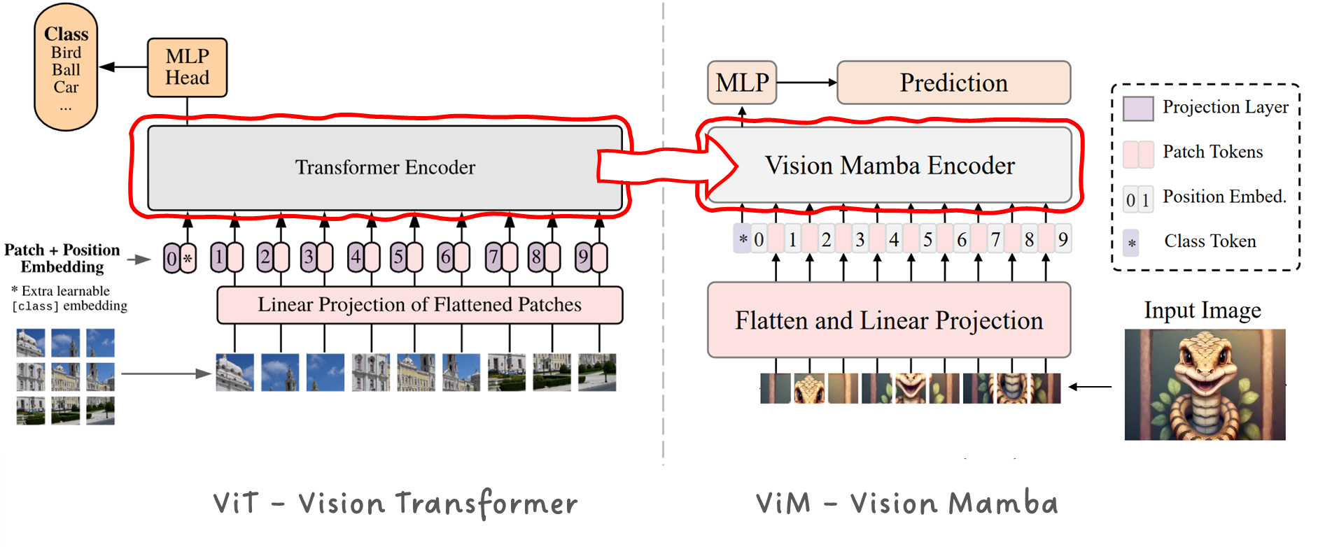 Image 7: Comparing the ViT-Vision Transformer and the ViM-Vision Mamba models. Images taken from A. Dosovitskiy et. al. and L. Zhu et. al., annotated by Sascha Kirch.
Vision Mamba aims to define a new generic vision backbone using Mamba state space models.
To represent an image as a sequence, because Mamba is still a sequence-to-sequence model after all, it is divided into patches, unrolled and then linearly projected and combined with positional encodings before fed into a stack of Mamba Encoder Blocks. The linearly scaling law of Mamba is especially interesting for high resolution images. Because patching the image as introduced in the ViT was a direct consequence of the O(N²) complexity of the attention block in the Transformer. With Mamba having an O(N) complexity, either smaller patches or higher resolutions can be processed for a fraction of the compute resources. In fact, without any attention mechanism involved, Vision Mamba was 2.8x faster than DeiT (Data efficient Vision Transformer) and saves up to 86.8% GPU memory on images of resolution 1024x1024.
Unlike most time signals, where each new sample has a causal relationship with its past samples, an image does not has this property. In images we do have long range dependencies between various pixel positions before and after the current pixel. To deal with this non-causal representation, Vision Mamba introduces a bidirectional Encoder Block, that includes two SSMs: one that is inferred with the normal sequence and one that is inferred on the inverted sequence.
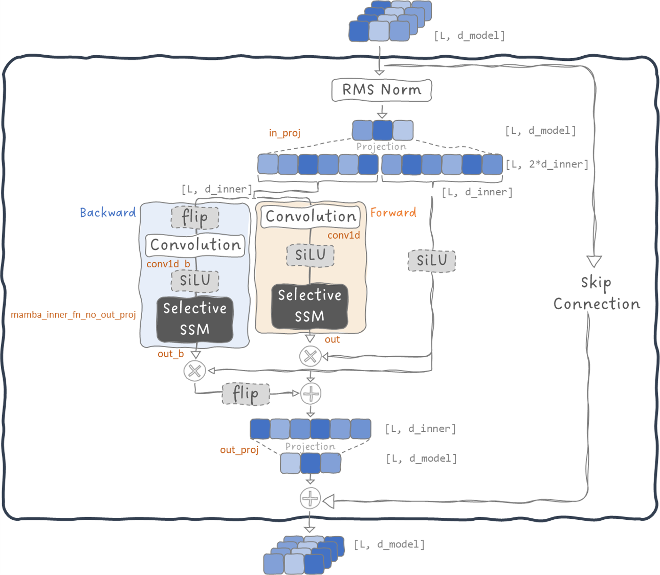 Image 8: Detailed block diagram of the Mamba-Block used in the ViM - Vision Mamba Encoder model. Image by Sascha Kirch.
👉 What you will find in part 4:
We will take a closer look on how to transform an image into a sequence. We will talk about the main motivation of the patchification and check how Mamba can handle smaller patches. We'll further review the insertion of the positional embeddings and the CLS token. Finally, we will talk about the bidirectional MambaBlock, what its intensions are and how it is implemented. We close part 4 with interpreting the experiments to see how it compares to previous methods.
Vision Mamba: Like a Vision Transformer but Better
6. VideoMamba - Understanding Videos
A primer for part 5 of this series
Mamba had to catch up very fast with the current developments of deep learning. Having more compute resources, data and foundation models as ever before, deep learning tackles data modalities previously thought to be too complex to handle. So, it was just a question off time how long it takes for Mamba to tackle videos (and this time was less than 2 Months after the ViM was published on arxiv).
VideoMamba is the extension of Vision Mamba but applied on videos. It classifies videos instead of images.
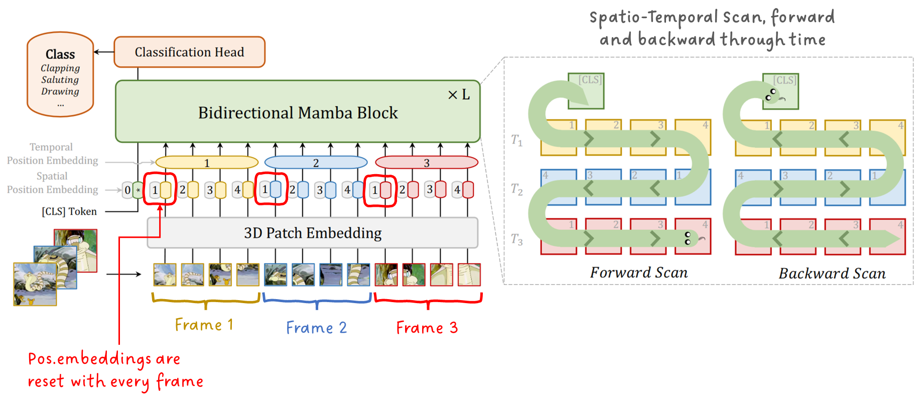 Image 9: Architecture of VideoMamba. Image by K. Li et al., annotated by Sascha Kirch.
Videos add an extra temporal dimension to the input data. Previous methods used 3D convolutions or Transformers to tackle videos, but both are very expensive computationally and in terms of memory usage. Not only does video introduces long range dependencies through time, but video is also very redundant, since between frames, pixels often do not change or do only change slightly (imagine a scene containing a blue sky). One trick to deal with these redundancies was key frame extraction to reduce the number of frames that needed to be processed. Again, Mamba with its linear complexity of O(N) comes in handy.
The architecture of VideoMamba is very similar to Vision Mamba. It patchifies the input, does a linear projection and adds positional encodings before feeding it into the Mamba Block. Now take a closer look onto the positional embeddings. The index of the spatial positional embedding for the patches is reset with every frame and each frame gets an extra temporal positional embedding that is constant for all patches within a frame.
Remember that for Vision Mamba the bidirectional block was introduced to deal with the non-causal relationships of pixels within a given frame. As you can imagine, this becomes even more complex when adding an extra temporal dimension. In their experiments they showed it works better to first scan through the spatial dimensions before tackling the temporal dimensions.
👉 What you will find in part 5:
We start part 5 with a general overview of the model architecture and how it has evolved from Vision Mamba. We then take a closer look onto the positional embeddings and the different scanning directions of the spatiotemporal inputs. We will talk about how VideoMamba avoids overfitting through a self-distillation mechanism and we will find out how short-term actions and long range dependencies are improved.
Paper Walkthroughs by Sascha Kirch
7. MambaMixer - Adding Selectivity to Channels
A primer for part 6 of this series
One minor detail we haven't mentioned yet in this article: Mamba and its variants apply the SSM to each channel individualy. This means information cannot flow from one channel to another. Or put differently: there is no selection between channels which limits Mamba's ability to find relationships in multi-dimensional data (e.g. images with their 3 color channels) or multi-variate time signals.
MambaMixer solves this issue by a neat little trick: it transposes the feature map before feeding it through a second SSM:
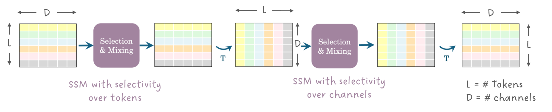 Image 10: Effect of transposing the input matrix. Image by A. Behrouz et.al., annotated by Sascha Kirch.
In that way the SSM is first applied over the token axis and is then applied over the channel axis. The individual blocks are called the TokenMixer and the ChannelMixer respectively. Both, the TokenMixer and the ChannelMixer combined build the MambaMixer Block.
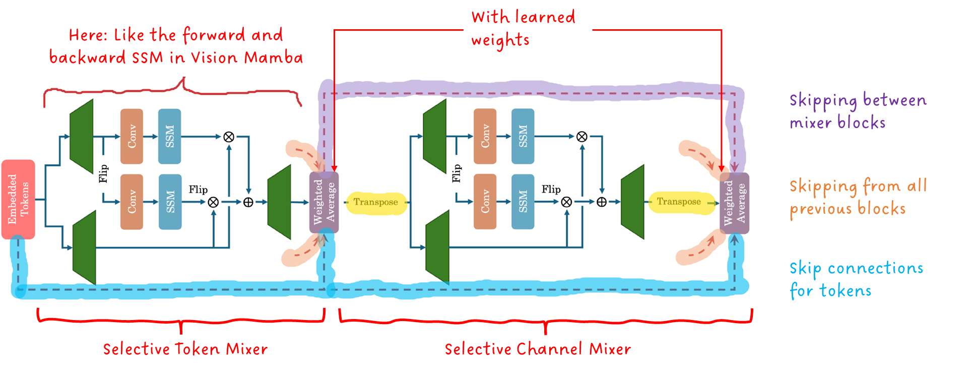 Image 11: General architecture of a MambaMixer Block. Image by A. Behrouz et.al., annotated by Sascha Kirch.
Each block can in theory have multiple SMMs for different scanning directions over the input patches. Multiple MambaMixerBlocks are stacked to build the MambaMixer. To further improve the performance and the training stability, outputs from previous TokenMixer and ChannelMixer blocks are combined via a learned weighted average.
In the Paper they build two models using the MambaMixer Block: Vision MambaMixer (ViM2) and Time Series MambaMixer (TSM2). As the Name suggest ViM2 is applied on images and TSM2 on multi-variate time series.
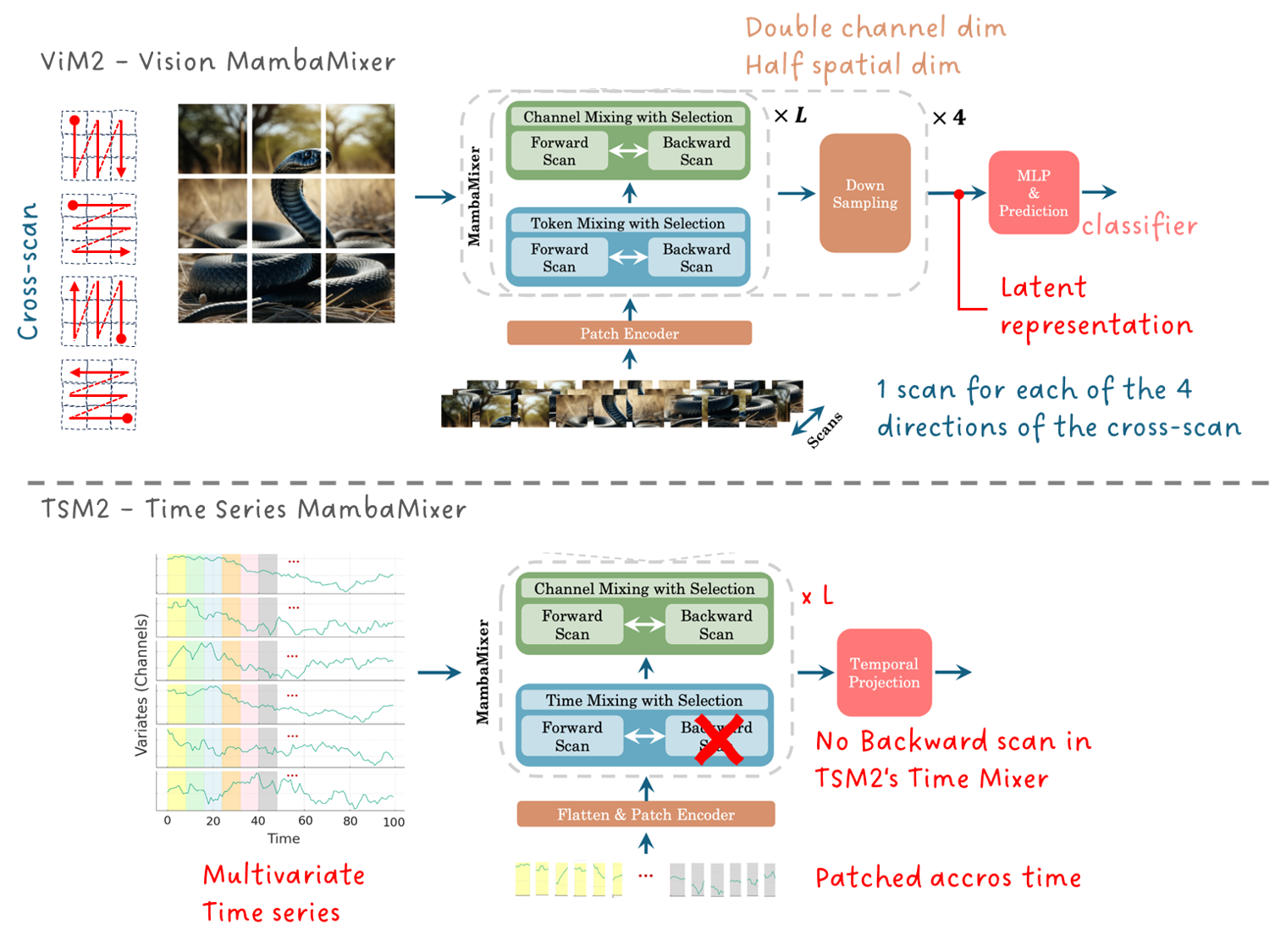 Image 12: Architecture of the ViM2 (Vision MambaMixer) and the TSM2 (Time Series MambaMixer). Image by A. Behrouz et.al., annotated by Sascha Kirch.
This paper is strongly inspired by the MLP Mixer Paper that aimed to simplify the architecture of the Vision Transformer (ViT). Here the friend-link to my post where I briefly introduced the MLP Mixer:
MLP Mixer in a Nutshell
👉 What you will find in part 6:
We start part 6 by motivating the issue of not exchanging information between different channels. We then take a closer look onto the general architecture that achieves selectivity for tokens and for channels. After that, we inspect the two proposed implementations using the MambaMixer that resulted in the ViM2 and the TSM2 architecture.
8. Mamba-2 - Closing the Gap Between Attention and SSMs
A primer for part 7 of this series
So far Mamba has been applied very successful to various applications and data modalities. It has been a strong competitor to the Transformer architecture surpassing the Transformer in some of the tasks and benchmarks. Still, SSMs suffer from some drawbacks: They are up against a deep learning infrastructure specifically tailored towards the Transfomer and its attention mechanism. In addition, Mamba's selective parallel scan does not leverage the matrix multiplication units of modern GPUs.
Mamba-2 aims to reformulate the SSM to show the duality with the attention mechanism to leverage this optimized ecosystem and to take advantage of fast matrix multiplication units of modern hardware accelerators.
Specifically, if the SSM is formulated in terms of a TxT semiseparable matrix, one can achieve exactly that.
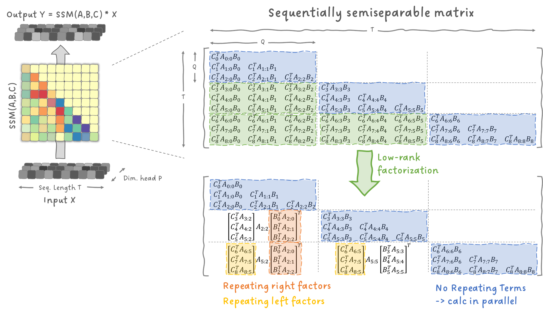 Image 13: SSMs as semiseparable matrix. Image by Sascha Kirch.
The calculation of the output Y becomes a matrix multiplication of the input X and the SSM, which is defined by the matrices A , B and C , that form a semiseparable matrix. Having such a matrix allows block decomposition, meaning, one can divide the matrix into sub-matrices of dimensions QxQ.
The resulting blocks on the diagonal are triangular matrices. None of those blocks share the same entries, meaning they can all be computed in parallel. The blocks off-diagonal can further be simplified using a low-rank factorization. Note that the same factors apear in multiple blocks, meaning they only need to be calculated once and can then be reused, allowing further speed up.
By defining this state space duality (SSD), the authors were able to
- show the connection between SSMs and attention,
- reformulate the SSM using semiseparable matrix transformations which in turn allows the implementation of a faster algorithm that uses less memory and takes advantage of the GPU's dedicated matrix multiplication cores,
- design of the new Mamba-2 Block that also allows to apply modern parallelization techniques such as tensor parallelism or sequence parallelism,
- introduce various analog concepts of prominent multi-head patterns in Transformers to SSMs like for example the multi-head SSM (MHS).
To conclude, the SSD framework ends up having a smaller memory footprint as attention and the SSM and is 2x-8x faster as the SSM since it uses matrix multiplication in the core of its formulation.
👉 What you will find in part 7:
In Part 7 we will revisit why having semiseparable matrices improves speed and memory footprint. We will also see, that the low-rank factorization can be interpreted as a state space model and how we can leverage modern hardware accelerators. We will further learn about the Mamba-2 block, and how it enables prominent parallelization techniques. And of course, you'll learn about the multi-head patterns that can be achieved.
9. Conclusion
Mamba state space models are a promising alternative to Transformers and RNNs to build a new generation general purpose architecture that can be applied to any data modality.
Within a short amount of time, Mamba-like models have been successfully applied to many problems in deep learning.
The close connection to system theory, the advanced algebra involved and the fact that modern deep learning ecosystems are tailored towards the Transformer might be an obstacle for researchers to adopt this new family of models. But thanks to the hard work and dedication of some researchers, Mamba-like models are becoming increasingly faster and more efficient on modern hardware accelerators and its integration into standard deep learning layers makes it increasingly easier to include into your own project.
Thank You!
🤝 I'd like to thank you, t he readers of my stories, for your constant support, clapping for my stories and, following me to never miss any of my latest articles. It is you who motivates me to continue writing, dive deep into complex topics, and become a better engineer/researcher by writing about them. You are awesome!
Continue Reading Part 2
Structured State Space Models Visually Explained
Further Readings & Resources
Mamba State Space Models for Images, Videos and Time Series
Paper Walkthroughs by Sascha Kirch
Blog Posts
Papers:
- S4: Efficiently Modeling Long Sequences with Structured State Spaces by A. Gu et.al., 31 Oct. 2021
- Mamba: Linear-Time Sequence Modeling with Selective State Spaces by A. Gu et.al., 1 Dec. 2023
- Vision Mamba: Efficient Visual Representation Learning with Bidirectional State Space Model by L. Zhu et.al., 17 Jan. 2024
- VideoMamba: State Space Model for Efficient Video Understanding by K. Li et.al., 11 Mar. 2024
- MambaMixer: Efficient Selective State Space Models with Dual Token and Channel Selection by A. Behrouz et.al., 29 Mar. 2024
- Mamba-2: Transformers are SSMs: Generalized Models and Efficient Algorithms Through Structured State Space Duality by A. Gu et.al., 31 May 2024
- S5: Simplified State Space Layers for Sequence Modeling by J. Smith et.al., 9 Aug. 2022
- HiPPO: Recurrent Memory with Optimal Polynomial Projections by A. Gu et.al., 17 Aug. 2020
- LSSL: Combining Recurrent, Convolutional, and Continuous-time Models with Linear State-Space Layers by A. Gu et.al., 26 Oct. 2021
- DSS: Diagonal State Spaces are as Effective as Structured State Spaces by A. Gupta et.al., 27 Mar. 2022
- S4D: On the Parameterization and Initialization of Diagonal State Space Models by A. Gu et.al., 23 Jun. 2022
- The Hidden Attention of Mamba Models by A. Ali et.al., 3 Mar 2024
Register Now to Continue Reading
Unlock Towards Data Science with a Free Account
All articles on Towards Data Science are available to registered users. Create a free account today to access this article and thousands more.
Register for freeSign in to your account
 Written By
See all from Sascha Kirch
Deep DivesDeep LearningMamba Image Video SignalState Space ModelTransformers
Share This Article
Towards Data Science is a community publication. Submit your insights to reach our global audience and earn through the TDS Author Payment Program.
Write for TDS
Related Articles
Deep Learning
Is one of them really better than the other? An explanation from a ML engineer who uses both frameworks.
Nour Islam Mokhtari
August 1, 20215 min read
Deep Learning
A review of techniques for modeling whole slide histology images and recommendations for different situations.
Heather Couture
March 31, 202112 min read
Artificial Intelligence
Learn how to create AI Agents using the OpenAI Agents SDK to automate Jira ticket creation from a meeting transcript.
Juan Carlos Suarez
July 24, 202514 min read
Artificial Intelligence
How can an LLM be applied effectively for biomedical entity linking?
Anand Subramanian
March 19, 202427 min read
Math
Mathematics, Hamiltonian Monte Carlo, generative models, and research frontiers ✨
Soran Ghaderi
March 28, 202515 min read
Deep Learning
Why L0.5, L3, and L4 Regularizations Are Uncommon
Amy Ma
November 29, 20236 min read
Deep Learning
The full code for this is available on my Github at https://github.com/jameslawlor/kaggle_galaxy_zoo.
James
July 12, 20175 min read
Artificial Intelligence
Apple Silicon has brought impressive performance gains with great power efficiency. Can we use these chips for Deep Learning as well?
Jiří Moravčík
March 1, 20244 min read
Artificial Intelligence
Based on my experience.
Davide Giordano
July 25, 20205 min read
Your home for data science and AI. The world's leading publication for data science, data analytics, data engineering, machine learning, and artificial intelligence professionals.
Subscribe to Our NewsletterWrite For TDS•About•Advertise•Privacy Policy•Terms of Use
© Insight Media Group, LLC 2026•The New Stack•roadmap.sh•Creator Network
Recommended Articles
Close
word word word word word word word word word word word word word word word word word word word word word word word word word word word word word word word word word word word word word word word word word word word word word word word word word word word word word word word word word word word word word word word word word word word word word word word word word word word word word word word word word word word word word word word word word word word word word word word word word word word word word word word word word word word word word word word word word word word word word word word word word word word word word word word word word word word word word word word word word word word word word word word word word word word word word word word word word word word word word word word word word word word word word word word word word word word word word word word word word word word word word word word word word word word word word word word word word word word word word word word word
mmMwWLliI0fiflO&1
mmMwWLliI0fiflO&1
mmMwWLliI0fiflO&1
mmMwWLliI0fiflO&1
mmMwWLliI0fiflO&1
mmMwWLliI0fiflO&1
mmMwWLliI0fiflO&1