保留正文与补采附件。源页面当前未重新核验;具体限制见交付清单。
 We value your privacy
We use cookies to enhance your browsing experience, serve personalised ads or content, and analyse our traffic. By clicking "Accept All", you consent to our use of cookies.
Customise Reject All Accept All
Customise Consent Preferences
 We use cookies to help you navigate efficiently and perform certain functions. You will find detailed information about all cookies under each consent category below.
The cookies that are categorised as "Necessary" are stored on your browser as they are essential for enabling the basic functionalities of the site. ... Show more
NecessaryAlways Active
Necessary cookies are required to enable the basic features of this site, such as providing secure log-in or adjusting your consent preferences. These cookies do not store any personally identifiable data.
-
Cookie
BCTempID
-
Duration
10 minutes
-
Description
No description available.
-
Cookie
__cf_bm
-
Duration
1 hour
-
Description
This cookie, set by Cloudflare, is used to support Cloudflare Bot Management.
-
Cookie
AWSALBCORS
-
Duration
7 days
-
Description
Amazon Web Services set this cookie for load balancing.
-
Cookie
_cfuvid
-
Duration
session
-
Description
Cloudflare sets this cookie to track users across sessions to optimize user experience by maintaining session consistency and providing personalized services
-
Cookie
li_gc
-
Duration
6 months
-
Description
Linkedin set this cookie for storing visitor's consent regarding using cookies for non-essential purposes.
-
Cookie
__hssrc
-
Duration
session
-
Description
This cookie is set by Hubspot whenever it changes the session cookie. The __hssrc cookie set to 1 indicates that the user has restarted the browser, and if the cookie does not exist, it is assumed to be a new session.
-
Cookie
__hssc
-
Duration
1 hour
-
Description
HubSpot sets this cookie to keep track of sessions and to determine if HubSpot should increment the session number and timestamps in the __hstc cookie.
-
Cookie
wpEmojiSettingsSupports
-
Duration
session
-
Description
WordPress sets this cookie when a user interacts with emojis on a WordPress site. It helps determine if the user's browser can display emojis properly.
-
Cookie
BCSessionID
-
Duration
1 year 1 month 4 days
-
Description
Blueconic sets this cookie as a unique identifier for the BlueConic profile.
-
Cookie
_octo
-
Duration
1 year
-
Description
No description available.
-
Cookie
logged_in
-
Duration
1 year
-
Description
No description available.
-
Cookie
__Secure-YEC
-
Duration
past
-
Description
YouTube sets this cookie to stores the user's video player preferences using embedded YouTube video
-
Cookie
__eoi
-
Duration
6 months
-
Description
Description is currently not available.
-
Cookie
AWSALBTGCORS
-
Duration
7 days
-
Description
No description available.
-
Cookie
login-status-p
-
Duration
past
-
Description
Description is currently not available.
-
Cookie
AWSALBTG
-
Duration
7 days
-
Description
No description available.
-
Cookie
csrf_token
-
Duration
session
-
Description
No description available.
-
Cookie
token_v2
-
Duration
1 day
-
Description
Description is currently not available.
-
Cookie
D
-
Duration
1 year
-
Description
Description is currently not available.
-
Cookie
PHPSESSID
-
Duration
session
-
Description
This cookie is native to PHP applications. The cookie stores and identifies a user's unique session ID to manage user sessions on the website. The cookie is a session cookie and will be deleted when all the browser windows are closed.
-
Cookie
VISITOR_PRIVACY_METADATA
-
Duration
6 months
-
Description
YouTube sets this cookie to store the user's cookie consent state for the current domain.
-
Cookie
cookietest
-
Duration
session
-
Description
The cookietest cookie is typically used to determine whether the user's browser accepts cookies, essential for website functionality and user experience.
-
Cookie
__Host-airtable-session
-
Duration
1 year
-
Description
This cookie is used to enable us to integrate the services of Airtable.
-
Cookie
__Host-airtable-session.sig
-
Duration
1 year
-
Description
This cookie is used to enable us to integrate the services of Airtable.
-
Cookie
m
-
Duration
1 year 1 month 4 days
-
Description
Stripe sets this cookie for fraud prevention purposes. It identifies the device used to access the website, allowing the website to be formatted accordingly.
-
Cookie
BIGipServer*
-
Duration
session
-
Description
Marketo sets this cookie to collect information about the user's online activity and build a profile about their interests to provide advertisements relevant to the user.
-
Cookie
__cfruid
-
Duration
session
-
Description
Cloudflare sets this cookie to identify trusted web traffic.
-
Cookie
_GRECAPTCHA
-
Duration
6 months
-
Description
Google Recaptcha service sets this cookie to identify bots to protect the website against malicious spam attacks.
-
Cookie
__Secure-YNID
-
Duration
6 months
-
Description
Google cookie used to protect user security and prevent fraud, especially during the login process.
-
Cookie
cookieyes-consent
-
Duration
1 year
-
Description
CookieYes sets this cookie to remember users' consent preferences so that their preferences are respected on subsequent visits to this site. It does not collect or store any personal information about the site visitors.
Functional
Functional cookies help perform certain functionalities like sharing the content of the website on social media platforms, collecting feedback, and other third-party features.
-
Cookie
lidc
-
Duration
1 day
-
Description
LinkedIn sets the lidc cookie to facilitate data center selection.
-
Cookie
brw
-
Duration
1 year
-
Description
No description available.
-
Cookie
brwConsent
-
Duration
5 minutes
-
Description
Description is currently not available.
-
Cookie
WMF-Uniq
-
Duration
1 year
-
Description
Description is currently not available.
-
Cookie
loom_anon_comment
-
Duration
1 year
-
Description
No description available.
-
Cookie
loom_referral_video
-
Duration
session
-
Description
Description is currently not available.
-
Cookie
VISITOR_INFO1_LIVE
-
Duration
6 months
-
Description
A cookie set by YouTube to measure bandwidth that determines whether the user gets the new or old player interface.
-
Cookie
yt-remote-connected-devices
-
Duration
Never Expires
-
Description
YouTube sets this cookie to store the user's video preferences using embedded YouTube videos.
-
Cookie
ytidb::LAST_RESULT_ENTRY_KEY
-
Duration
Never Expires
-
Description
The cookie ytidb::LAST_RESULT_ENTRY_KEY is used by YouTube to store the last search result entry that was clicked by the user. This information is used to improve the user experience by providing more relevant search results in the future.
-
Cookie
yt-remote-device-id
-
Duration
Never Expires
-
Description
YouTube sets this cookie to store the user's video preferences using embedded YouTube videos.
-
Cookie
yt-remote-session-name
-
Duration
session
-
Description
The yt-remote-session-name cookie is used by YouTube to store the user's video player preferences using embedded YouTube video.
-
Cookie
yt-remote-fast-check-period
-
Duration
session
-
Description
The yt-remote-fast-check-period cookie is used by YouTube to store the user's video player preferences for embedded YouTube videos.
-
Cookie
yt-remote-session-app
-
Duration
session
-
Description
The yt-remote-session-app cookie is used by YouTube to store user preferences and information about the interface of the embedded YouTube video player.
-
Cookie
yt-remote-cast-available
-
Duration
session
-
Description
The yt-remote-cast-available cookie is used to store the user's preferences regarding whether casting is available on their YouTube video player.
-
Cookie
yt-remote-cast-installed
-
Duration
session
-
Description
The yt-remote-cast-installed cookie is used to store the user's video player preferences using embedded YouTube video.
-
Cookie
cp_session
-
Duration
3 months
-
Description
Codepen sets this cookie for Help systems found in the website.
-
Cookie
loid
-
Duration
1 year 1 month 4 days
-
Description
This cookie is set by the Reddit. The cookie enables the sharing of content from the website onto the social media platform.
Analytics
Analytical cookies are used to understand how visitors interact with the website. These cookies help provide information on metrics such as the number of visitors, bounce rate, traffic source, etc.
-
Cookie
__hstc
-
Duration
6 months
-
Description
Hubspot set this main cookie for tracking visitors. It contains the domain, initial timestamp (first visit), last timestamp (last visit), current timestamp (this visit), and session number (increments for each subsequent session).
-
Cookie
hubspotutk
-
Duration
6 months
-
Description
HubSpot sets this cookie to keep track of the visitors to the website. This cookie is passed to HubSpot on form submission and used when deduplicating contacts.
-
Cookie
_ga
-
Duration
1 year 1 month 4 days
-
Description
Google Analytics sets this cookie to calculate visitor, session and campaign data and track site usage for the site's analytics report. The cookie stores information anonymously and assigns a randomly generated number to recognise unique visitors.
-
Cookie
ga*
-
Duration
1 year 1 month 4 days
-
Description
Google Analytics sets this cookie to store and count page views.
-
Cookie
__Host-psifi.analyticsTrace
-
Duration
6 hours
-
Description
Description is currently not available.
-
Cookie
__Host-psifi.analyticsTraceV2
-
Duration
6 hours
-
Description
Description is currently not available.
-
Cookie
_gh_sess
-
Duration
session
-
Description
GitHub sets this cookie for temporary application and framework state between pages like what step the user is on in a multiple step form.
-
Cookie
YSC
-
Duration
session
-
Description
YSC cookie is set by Youtube and is used to track the views of embedded videos on Youtube pages.
-
Cookie
ajs_anonymous_id
-
Duration
1 year
-
Description
This cookie is set by Segment to count the number of people who visit a certain site by tracking if they have visited before.
-
Cookie
vuid
-
Duration
1 year 1 month 4 days
-
Description
Vimeo installs this cookie to collect tracking information by setting a unique ID to embed videos on the website.
Performance
Performance cookies are used to understand and analyse the key performance indexes of the website which helps in delivering a better user experience for the visitors.
-
Cookie
AWSALB
-
Duration
7 days
-
Description
AWSALB is an application load balancer cookie set by Amazon Web Services to map the session to the target.
-
Cookie
acq
-
Duration
past
-
Description
Description is currently not available.
-
Cookie
acq.sig
-
Duration
past
-
Description
Description is currently not available.
-
Cookie
ptc
-
Duration
2 years
-
Description
No description available.
Advertisement
Advertisement cookies are used to provide visitors with customised advertisements based on the pages you visited previously and to analyse the effectiveness of the ad campaigns.
-
Cookie
muc_ads
-
Duration
1 year 1 month 4 days
-
Description
Twitter sets this cookie to collect user behaviour and interaction data to optimize the website.
-
Cookie
guest_id_marketing
-
Duration
1 year 1 month 4 days
-
Description
Twitter sets this cookie to identify and track the website visitor.
-
Cookie
guest_id_ads
-
Duration
1 year 1 month 4 days
-
Description
Twitter sets this cookie to identify and track the website visitor.
-
Cookie
personalization_id
-
Duration
1 year 1 month 4 days
-
Description
Twitter sets this cookie to integrate and share features for social media and also store information about how the user uses the website, for tracking and targeting.
-
Cookie
guest_id
-
Duration
1 year 1 month 4 days
-
Description
Twitter sets this cookie to identify and track the website visitor. It registers if a user is signed in to the Twitter platform and collects information about ad preferences.
-
Cookie
bcookie
-
Duration
1 year
-
Description
LinkedIn sets this cookie from LinkedIn share buttons and ad tags to recognize browser IDs.
-
Cookie
__Secure-ROLLOUT_TOKEN
-
Duration
6 months
-
Description
YouTube sets this cookie to manage feature rollout and experimentation. It helps Google control which new features or interface changes are shown to users as part of testing and staged rollouts, ensuring consistent experience for a given user during an experiment.
-
Cookie
yt.innertube::nextId
-
Duration
Never Expires
-
Description
YouTube sets this cookie to register a unique ID to store data on what videos from YouTube the user has seen.
-
Cookie
yt.innertube::requests
-
Duration
Never Expires
-
Description
YouTube sets this cookie to register a unique ID to store data on what videos from YouTube the user has seen.
-
Cookie
session_tracker
-
Duration
session
-
Description
This cookie is set by the Reddit. This cookie is used to identify trusted web traffic. It also helps in adverstising on the website.
-
Cookie
edgebucket
-
Duration
session
-
Description
Reddit sets this cookie to save the information about a log-on Reddit user, for the purpose of advertisement recommendations and updating the content.
-
Cookie
did
-
Duration
1 year
-
Description
Arbor sets this cookie to show targeted ads to site visitors.This cookie expires after 2 months or 1 year.
Uncategorised
Other uncategorised cookies are those that are being analysed and have not been classified into a category as yet.
No cookies to display.
Reject All Save My Preferences Accept All
Toggle SearchToggle Mobile Navigation
Publish AI, ML & data-science insights to a global community of data professionals.
Sign inSubmit an Article
LatestEditor's PicksNewsletterShipAI
Write For TDS
LinkedInXToggle Search
Deep Learning
Why Data Scientists Can't Afford Too Many Dimensions and What They Can Do About It
An in-depth article about dimensionality reduction and its most popular methods
Niklas Lang
January 16, 202514 min read
 Photo by Paulina Gasteiger on Unsplash
Dimensionality reduction is a central method in the field of Data Analysis and Machine Learning that makes it possible to reduce the number of dimensions in a data set while retaining as much of the information it contains as possible. This step is necessary to reduce the dimensionality of the dataset before training to save computing power and avoid the problem of overfitting.
In this article, we take a detailed look at dimensionality reduction and its objectives. We also illustrate the most commonly used methods and highlight the challenges of dimensionality reduction.
Learn this step by step with the interactive Machine Learning roadmap.
What is Dimensionality Reduction?
Dimensionality reduction comprises various methods that aim to reduce the number of characteristics and variables in a data set while preserving the information in it. In other words, fewer dimensions should enable a simplified representation of the data without losing patterns and structures within the data. This can significantly accelerate downstream analyses and also optimize machine learning models.
In many applications, problems occur due to the high number of variables in a data set, which is also referred to as the curse of dimensionality. For example, too much dimensionality can lead to these problems:
- Overfitting: When machine learning models become overly reliant on characteristics of the training dataset and therefore only provide poor results for new, unseen data, this is known as overfitting. With a high number of features, the risk of overfitting increases as the model becomes more complex and therefore adapts too strongly to the errors in the data set.
- Computational complexity : Analyses and models that have to process many variables often require more parameters to be trained. This increases the computational complexity, which is reflected either in a longer training time or in increased resource consumption.
- Data Noise : With an increased number of variables, the probability of erroneous data or so-called noise also increases. This can influence the analyses and lead to incorrect predictions.
Although large data sets with many characteristics are very informative and valuable, the high number of dimensions can also quickly lead to problems. Dimensionality reduction is a method that attempts to preserve the information content of the data set while reducing the number of dimensions.
What is the Curse of Dimensionality?
The Curse of Dimensionality occurs with high-dimensional data sets, i.e. those that have a large number of attributes or features. At first, many attributes are a good thing because they contain a lot of information and describe the data points well. For example, if we have a dataset about people, the attributes can be information such as hair color, height, weight, eye color, etc.
In mathematical terms, however, each additional attribute means a new dimension in the space and therefore a significant increase in possibilities. This becomes clear from the following example, in which we want to find out which customers buy which products. In the first step, we only look at the age of the prospective customers and whether they have bought the product. We can still depict this relatively easily in a two-dimensional diagram.
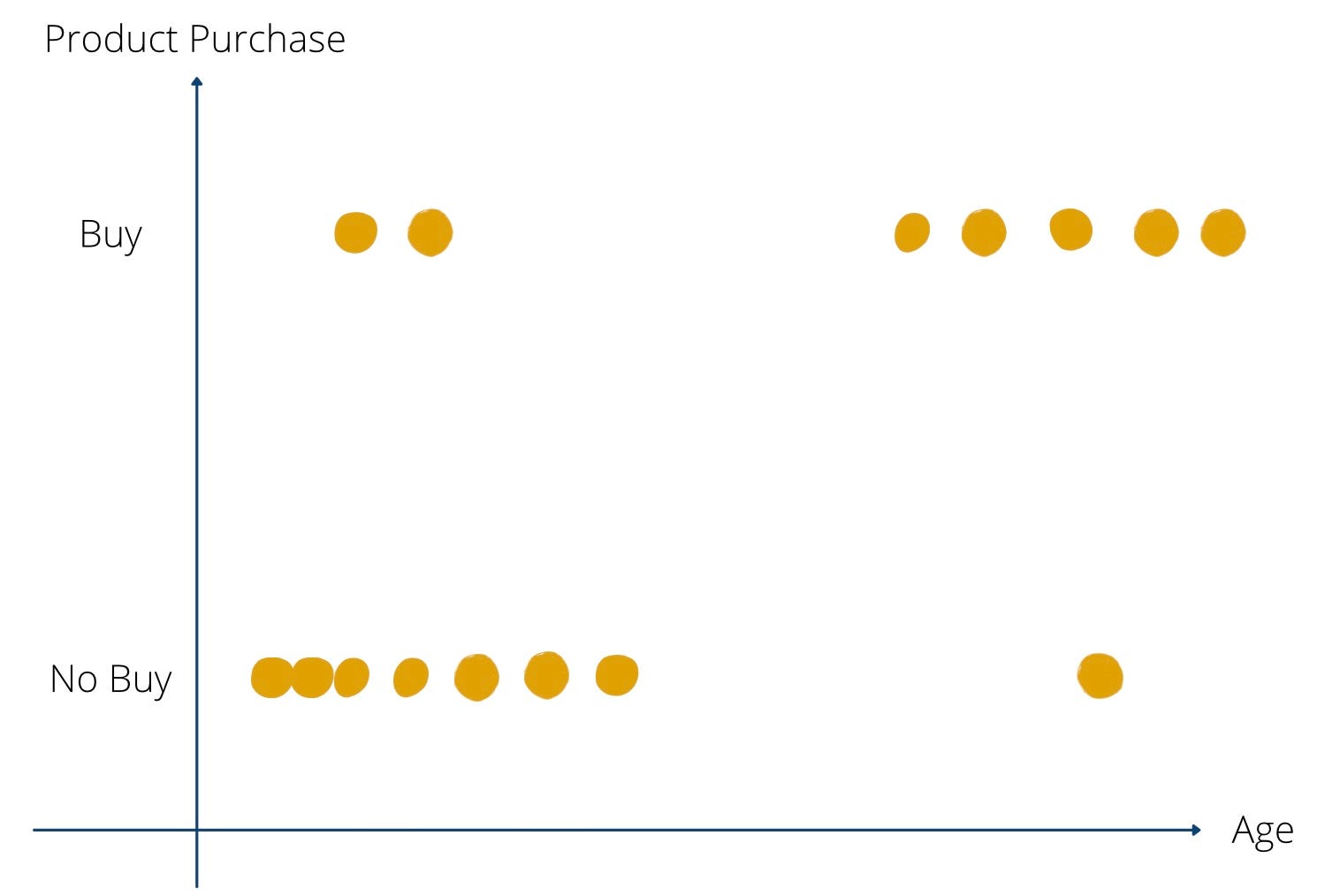 Diagram of Buyers divided by Age | Source: Author
As soon as we add more information about the customer, things get a little more complex. The information on the customer's income would mean a new axis on which the numerical income is mapped. So the two-dimensional diagram becomes a three-dimensional one. The additional attribute "gender" would lead to a fourth dimension and so on.
When working with data, it is desirable to have a lot of attributes and information in the data set to give the model many opportunities to recognize structures in the data. However, it can also lead to serious problems, as the name Curse of Dimensionality suggests.
Data Sparsity
The example shown illustrates a problem that occurs with many attributes. Due to the large number of dimensions, the so-called data space, i.e. the number of values a dataset can take on, also grows. This can lead to what is known as data sparsity meaning that the training data set used to train the model does not contain certain values at all or only very rarely. As a result, the model only delivers poor results for these marginal cases.
Let's assume that we examine 1,000 customers in our example, as it would be too time-consuming to survey even more customers or this data is simply not available. All age groups from young to old may be well represented among these customers. However, if the additional dimension of income is added, it becomes less likely that the possible characteristics, such as "young" and "high income" or "old" and "medium income", will occur and be backed up with enough data points.
Distance Concentration
If you want to evaluate the similarity of different data sets in the field of machine learning, distance functions are often used for this. The most common clustering algorithms, such as k-means clustering, rely on calculating the distance between points and assigning them to a cluster depending on their size. In multidimensional spaces, however, it can quickly become the case that all points are at a similar distance from each other so it seems almost impossible to separate them.
We are also familiar with this phenomenon from everyday life. If you take a photo of two objects, such as two trees, they can look very close to each other in the picture, as it is only a two-dimensional image. In real life, however, the trees may be several meters apart, which only becomes clear in three dimensions.
All these problems, which can occur in connection with many dimensions, are summarized under the term Curse of Dimensionality.
What are the Goals of Dimensionality Reduction?
Dimensionality reduction primarily pursues three primary goals: Improving model performance, visualizing data, and increasing processing speed. We will examine these in more detail in the following section.
Improving Model Performance
One of the main goals of dimensionality reduction is to improve model performance. By reducing the number of variables in a dataset, a less complex model can be used, which in turn reduces the risk of overfitting.
Models that have a large number of parameters and are therefore highly complex tend to overfit the training dataset and the noise in the data. As a result, the model delivers poorer results with new data that does not contain this noise, while the accuracy of the training data set is very good. This phenomenon is known as overfitting. During dimensionality reduction, unimportant or redundant features are removed from the data set, which reduces the risk of overfitting. As a result, the model delivers better quality for new, unseen data.
Visualization of Data
If you want to visualize data sets with many features, you face the challenge of mapping all this information in a two- or at most three-dimensional space. Any dimensionality beyond this is no longer directly tangible for us humans, but it is easiest to assign a separate dimension to each feature in the data set. Therefore, with high-dimensional data sets, we are often faced with the problem that we cannot simply visualize the data to gain an initial understanding of the peculiarities of the data and, for example, to recognize whether there are outliers.
Dimensionality reduction helps to reduce the number of dimensions to such an extent that visualization in two- or three-dimensional space is possible. This makes it easier to better understand the relationships between the variables and the data structures.
Increasing the Processing Speed
Computing time and the necessary resources play a major role in the implementation of projects, especially for machine learning and deep learning algorithms. Often, only limited resources are available, which should be used optimally. By removing redundant features from the data set at an early stage, you not only save time and computing power during data preparation but also when training the model, without having to accept lower performance.
In addition, dimensionality reduction makes it possible to use simpler models that not only require less power during initial training but can also perform calculations faster later during operation. This is an important factor, especially for real-time calculations.
Overall, dimensionality reduction is an important method for improving data analysis and building more robust machine-learning models. It is also an important step in the visualization of data.
Which Methods are used for Dimensionality Reduction?
In practice, various methods for dimensionality reduction have become established, three of which are explained in more detail below. Depending on the application and the structure of the data, these methods already cover a broad spectrum and can be used for most practical problems.
Principal Component Analysis
Principal component analysis (PCA) assumes that several variables in a data set possibly measure the same thing, i.e. are correlated. These different dimensions can be mathematically combined into so-called principal components without compromising the significance of the data set. The shoe size and height of a person, for example, are often correlated and can therefore be replaced by a common dimension to reduce the number of input variables.
Principal component analysis describes a method for mathematically calculating these components. The following two key concepts are central to this:
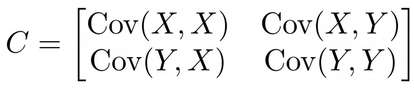
The covariance matrix is a matrix that specifies the pairwise covariances between two different dimensions of the data space. It is a square matrix, i.e. it has as many rows as columns. For any two dimensions, the covariance is calculated as follows:
 Here n stands for the number of data points in the data set, _X i is the value of the dimension X of the i -th data point and X̅ is the mean value of the dimension X for all n data points. As can be seen from the formula, the covariances between two dimensions do not depend on the order of the dimensions, so the following applies COV(X,Y) = COV(Y,X). These values result in the following covariance matrix C for the two dimensions X and Y :
 The covariance of two identical dimensions is simply the variance of the dimension itself, i.e:
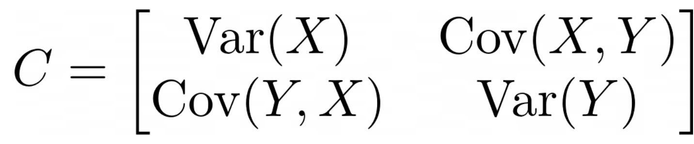 The covariance matrix is the first important step in the principal component analysis. Once this matrix has been created, the eigenvalues and eigenvectors can be calculated from it. Mathematically, the following equation is solved for the eigenvalues:
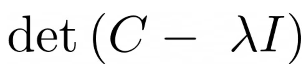 Here λ is the desired eigenvalue and I is the unit matrix of the same size as the covariance matrix C. When this equation is solved, one or more eigenvalues of a matrix are obtained. They represent the linear transformation of the matrix in the direction of the associated eigenvector. An associated eigenvector can therefore also be calculated for each eigenvalue, for which the slightly modified equation must be solved:
 Where v is the desired eigenvector, according to which the equation must be solved accordingly. In the case of the covariance matrix, the eigenvalue corresponds to the variance of the eigenvector, which in turn represents a principal component. Each eigenvector is therefore a mixture of different dimensions of the data set, the principal components. The corresponding eigenvalue therefore indicates how much variance of the data set is explained by the eigenvector. The higher this value, the more important the principal component is, as it contains a large proportion of the information in the data set.
Therefore, after calculating the eigenvalues, they are sorted by size and the eigenvalues with the highest values are selected. The corresponding eigenvectors are then calculated and used as principal components. This results in a dimension reduction, as only the principal components are used to train the model instead of the individual features of the data set.
t-Distributed Stochastic Neighbor Embedding (t-SNE)
t-Distributed Stochastic Neighbor Embedding, or t-SNE for short, approaches the problem of dimensionality reduction differently by attempting to create a new, lower-dimensional space that adopts the distances of the data points from the higher-dimensional space as far as possible. The basic idea of this becomes clear in the following example.
It is not easy to transfer data sets from a high dimensionality to a low dimensionality while retaining as much information as possible from the data set. The following figure shows a simple, two-dimensional data set with a total of 50 data points. Three different clusters can be identified, which are also well separated from each other. The yellow cluster is furthest away from the other two clusters, while the purple and blue data points are closer to each other.
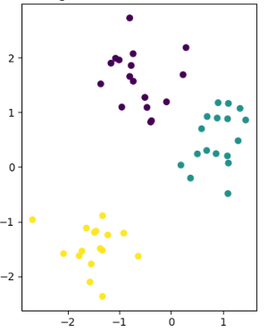 Two-dimensional data for t-SNE | Source: Author
The aim now is to convert this two-dimensional data set into a lower dimension, i.e. into one dimension. The simplest approach for this would be to represent the data either only by its X or Y coordinate.
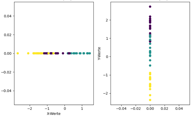 Dimensionality reduction by X- or Y-coordinate | Source: Author
However, it is clear that this simple transformation has lost much of the information in the data set and gives a different picture than the original two-dimensional data. If only the X coordinates are used, it looks as if the yellow and purple clusters overlap and that all three clusters are roughly equidistant from each other. If, on the other hand, only the Y coordinates are used for dimensionality reduction, the yellow cluster is much better separated from the other clusters, but it looks as if the purple and blue clusters overlap.
The basic idea of t-SNE is that the distances from the high dimensionality are transferred to the low dimensionality as far as possible. To do this, it uses a stochastic approach and converts the distances between points into a probability that indicates how likely it is that two random points are next to each other.
More precisely, it is a conditional probability that indicates how likely it is that one point would choose the other point as a neighbor. Hence the name "Stochastic Neighbor Embedding".
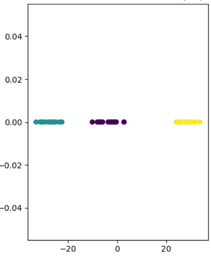 Dimensionality reduction according to t-SNE | Source: Author
As you can see, this approach leads to a much better result, in which the three different clusters can be clearly distinguished from one another. It is also clear that the yellow data points are significantly further away from the other data points and the blue and purple clusters are somewhat closer together. To better understand the details of this approach, you are welcome to read our detailed article on this topic.
Mastering t-SNE: A Comprehensive Guide to Understanding and Implementation in Python
Linear Discriminant Analysis
Linear Discriminant Analysis (LDA for short) aims to identify and maximize the separability between classes by projecting the data onto a smaller dimension. In contrast to other methods, it places particular emphasis on maximizing the separability between classes and is therefore particularly important for classification tasks.
Two central key figures are calculated:
- Within-Class Scatter : This key figure measures the variability within a class of data. The lower this value, the more similar the data points are within a class and the more the classes are separated.
- Between-class scatter : This scatter in turn measures the variability between the mean values of the classes. This value should be as large as possible, as this indicates that the classes are easier to separate from each other.
Simply put, these key figures are used to form matrices and calculate their eigenvalues. The eigenvectors for the largest eigenvalues are in turn the dimensions in the new feature space, which has fewer dimensions than the original data set. All data points can then be projected onto the eigenvectors, which reduces the dimensions.
Linear Discriminant Analysis is particularly suitable for applications in which the classes are already known and the data is also clearly labeled. It uses this class information from supervised learning to find a low-dimensional space that separates the classes as well as possible.
A disadvantage of LDA is that the maximum reduction to a dimensional space is limited and depends on the number of classes. A data set with (n) classes can therefore be reduced to a maximum of (n-1) dimensions. In concrete terms, this means, for example, that a data set with three different classes can be reduced to a two-dimensional space.
This approach of dimensionality reduction is also particularly suitable for large data sets, as the computing effort is only moderate and scales well with the amount of data so that the computing effort is kept within limits even with large amounts of data.
What are the Challenges of Dimensionality Reduction?
Dimensionality reduction is an important step in data pre-processing to increase the generalizability of machine learning models and the general model performance and possibly save computing power. However, the methods also bring with them some challenges that should be considered before use. These include
- Loss of information : Although the methods presented attempt to retain as much variance, i.e. information content, of the data set, some information is inevitably lost when dimensions are reduced. Important data can also be lost, which may lead to poorer analyses or model results. Therefore, the resulting model may be less accurate or less powerful.
- Interpretability : Most algorithms used for dimensionality reduction provide a low-dimensional space that no longer contains the original dimensions, but a mathematical summary of them. Principal component analysis, for example, uses the eigenvectors, which are a summary of various dimensions from the data set. As a result, interpretability is lost to a certain extent, as the previous dimensions are easier to measure and visualize. Especially in use cases where transparency is important and the results require a practical interpretation, this can be a decisive disadvantage.
- Scaling : Performing dimensionality reductions is computationally intensive and takes time, especially for large data sets. In real-time applications, however, this time is not available, as the computing time of the model is added to this. Computing-intensive models in particular, such as t-SNE or autoencoders, quickly fall out because they take too long to make live predictions.
- Selecting the method : Depending on the application, the dimensionality reduction methods presented have their strengths and weaknesses. The selection of a suitable algorithm therefore plays an important role, as it has a significant influence on the results. There is no one-size-fits-all solution and a new decision must always be made based on the application.
Dimensionality reduction has many advantages and is an integral part of data pre-processing in many applications. However, the disadvantages and challenges mentioned must also be taken into account to train an efficient model.
This is what you should take with you
- Dimensionality reduction is a method of reducing the number of dimensions, i.e. variables, in a data set while retaining as much information content as possible.
- With many input variables, the so-called curse of dimensionality arises. This leads to problems such as data sparsity or distance concentration.
- Dimensionality reduction often leads to a lower probability of overfitting, better visualization, and optimized computing power when training machine learning models.
- The most common dimensionality reduction methods include principal component analysis, t-SNE, and LDA.
- However, dimensionality reduction also has disadvantages, such as poorer interpretability or loss of information.
Register Now to Continue Reading
Unlock Towards Data Science with a Free Account
All articles on Towards Data Science are available to registered users. Create a free account today to access this article and thousands more.
Register for freeSign in to your account
 Written By
See all from Niklas Lang
Deep LearningDimensionality ReductionGetting StartedK Means ClusteringMachine Learning
Share This Article
Towards Data Science is a community publication. Submit your insights to reach our global audience and earn through the TDS Author Payment Program.
Write for TDS
Related Articles
Machine Learning
Fundamental statistic concepts to get you started on your Data Science journey
Terence Shin, MSc, MBA
January 13, 20205 min read
Machine Learning
Develop A Conceptual Understanding Of What It Means To Optimize A Portfolio
Tony Yiu
October 11, 20208 min read
Machine Learning
Grasp the idea behind credible and confidence interval in 5 minutes
Federico Comotto
February 7, 20225 min read
Machine Learning
Automated and easy-to-understand script to get the job done.
Dario Radečić
August 25, 20207 min read
Machine Learning
A step-by-step guide to the theory behind the beauty of closed-form solutions
Margo Hatcher
May 4, 20227 min read
Artificial Intelligence
We all learn from mistakes
Soner Yıldırım
September 19, 20214 min read
Artificial Intelligence
A great resource for all scientists.
Soner Yıldırım
August 6, 20203 min read
Artificial Intelligence
Introduction
Christophe Brown
November 11, 202110 min read
Deep Learning
Last part of the Transformer series
Chen Margalit
October 5, 20237 min read
Your home for data science and AI. The world's leading publication for data science, data analytics, data engineering, machine learning, and artificial intelligence professionals.
Subscribe to Our NewsletterWrite For TDS•About•Advertise•Privacy Policy•Terms of Use
© Insight Media Group, LLC 2026•The New Stack•roadmap.sh•Creator Network
Recommended Articles
Close