Assembling a GPT Model from Scratch

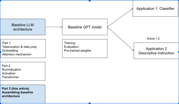
At this point, we have almost everything we need to assemble a baseline GPT model. In this article, I will:

Bring the different components together and show how they form the complete model.
Do a quick walkthrough of the tensor dimensions at each stage to understand how the data changes as it moves through the network.
Calculate the total number of trainable parameters in the model. This parameter count is typically what people refer to when they describe the size of a model.

Assembling the components

Let us begin with a quick review of the components introduced in the previous articles:

Tokenization and embeddings convert natural-language text into tokens and then represent those tokens as numerical vectors.
Attention allows each token to incorporate context from the other relevant tokens in the sequence.
Activation layers help the model identify and strengthen useful patterns within the data.
Normalization layers keep the values flowing through the model within a stable range.
Dropout layers randomly remove some information during training to reduce overfitting. I have left dropout out of the diagram below to keep it simple.

The following diagram represents how these components fit together in the baseline model:

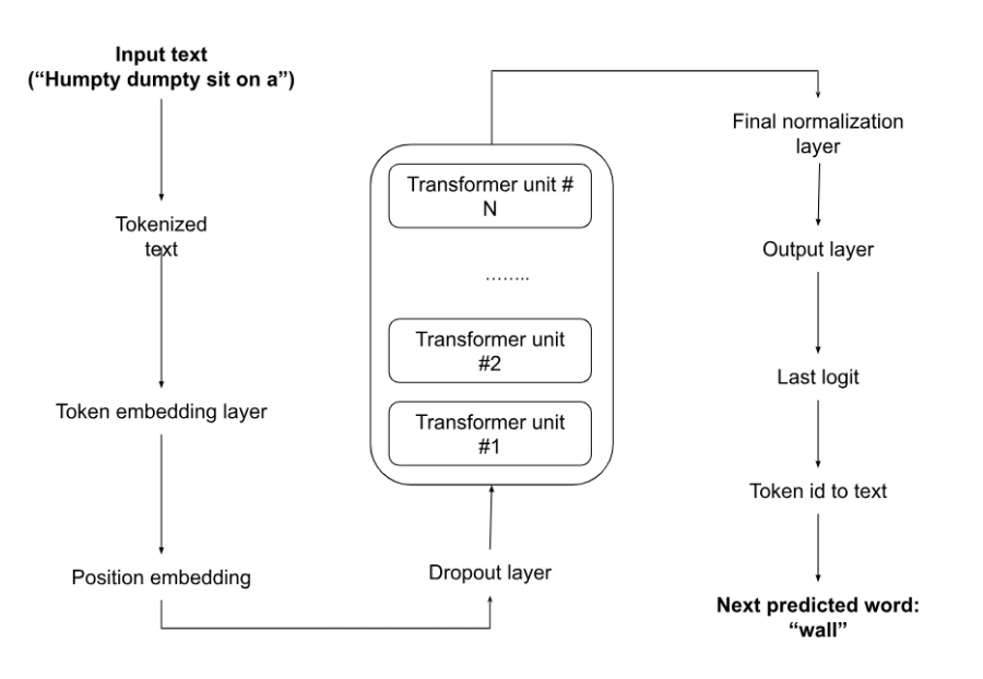
The following piece of code does the heavy lifting:

class GPTModel(nn.Module):
    def __init__(self, cfg):
        super().__init__()

        self.tok_emb = nn.Embedding(
            cfg["vocab_size"],
            cfg["emb_dim"]
        )
        self.pos_emb = nn.Embedding(
            cfg["context_length"],
            cfg["emb_dim"]
        )
        self.drop = nn.Dropout(cfg["drop_rate"])

        # Transformer block repeated n_layers times
        self.trf_blocks = nn.Sequential(
            *[
                TransformerBlock(cfg)
                for _ in range(cfg["n_layers"])
            ]
        )

        # Final normalization layer
        self.final_norm = LayerNorm(cfg["emb_dim"])
        self.out_head = nn.Linear(
            cfg["emb_dim"],
            cfg["vocab_size"],
            bias=False
        )

    def forward(self, in_idx):
        batch_size, seq_len = in_idx.shape

        tok_embeds = self.tok_emb(in_idx)
        pos_embeds = self.pos_emb(
            torch.arange(seq_len, device=in_idx.device)
        )

        x = self.drop(tok_embeds + pos_embeds)
        x = self.trf_blocks(x)
        x = self.final_norm(x)
        logits = self.out_head(x)

        return logits

Tracking tensor dimensions

Recall the model configuration introduced in Part 1:

GPT_CONFIG_124M = {
    "vocab_size": 50_257,
    "context_length": 1_024,
    "emb_dim": 768,
    "n_heads": 12,
    "n_layers": 12,
    "drop_rate": 0.1,
    "qkv_bias": False,
}

In addition, let us assume that every input has been padded or truncated to context_length and that each input batch contains batch_size inputs. Intuitively, the final output should give us batch_size predicted tokens—one for each input.

To keep things simple, we do not need to follow every tensor transformation inside the model. At a high level, the input begins as a sequence of token IDs. Each token is then converted into an emb_dim-dimensional vector, and this overall shape is preserved as the data moves through the transformer blocks.

Inside each block, the attention and activation components temporarily reshape or expand the data, but the output returns to the same dimensions.

Finally, the output layer converts each token representation into a score for every token in the vocabulary.

Stage	What happens	Output dimensions
Tokenization	Each input is converted into a sequence of token IDs.	`batch_size * context_length`
Token embeddings	Each token ID is converted into a vector in the embedding space.	`batch_size * context_length * emb_dim`
Positional embeddings	Position information is added to each token. The overall dimensions remain unchanged.	`batch_size * context_length * emb_dim`
Input to transformer blocks	Token and positional embeddings are combined and passed into the transformer blocks.	`batch_size * context_length * emb_dim`
Attention	The model creates query, key and value representations to understand relationships between tokens. The attention output returns to the original dimensions.	`batch_size * context_length * emb_dim`
Activation expansion	The representation is temporarily expanded to four times the embedding dimension.	`batch_size * context_length * (emb_dim * 4)`
Activation projection	The expanded representation is reduced back to the original embedding dimension.	`batch_size * context_length * emb_dim`
Output of each transformer block	The original tensor dimensions are preserved before the data enters the next block.	`batch_size * context_length * emb_dim`
Output layer	Each token representation is converted into a score for every token in the vocabulary.	`batch_size * context_length * vocab_size`
Final-position logits	The vocabulary scores from the final token position are selected for next-token prediction.	`batch_size * vocab_size`
Token prediction	One next token is selected for each input in the batch.	`batch_size * 1`

Count of trainable parameters

There is one final piece to examine before we complete the model: the total number of trainable parameters.

These are the values the model adjusts during training as it learns patterns from the data. The overall parameter count is also commonly used to describe the size of a model. For example, GPT-2 Small is referred to as a 124-million-parameter model.

Let us create an instance of our GPT model and count its parameters:

torch.manual_seed(123)
model = GPTModel(GPT_CONFIG_124M)

#setting output layer to use same weights as embedding layer. 
# as it is same dictionary. 
model.out_head.weight = model.tok_emb.weight


tied_param_count = sum(p.numel() for p in model.parameters())
print(f"Total number of unique parameters: {tied_param_count}")

The model produces the following output:


Total number of parameters: 124402944

Let us examine this in more detail:

Model component	Trainable parameters	How it is calculated
Token embeddings	38,597,376	`50,257 * 768`: one 768-dimensional embedding vector for each of the 50,257 tokens in the vocabulary
Positional embeddings	786,432	`1,024 * 768`: one 768-dimensional embedding vector for each of the 1,024 positions in the context window
12 transformer blocks	85,017,600	`7,084,800 * 12`: 12 transformer blocks, each containing attention, activation and normalization layers
Final normalization layer	1,536	`768 + 768`: one trainable scale value and one trainable shift value for each of the 768 embedding dimensions
Output head	0	re-using token embedding weights.
Total in the current implementation	124402944	Approximately 124 million parameters

Each transformer block contains approximately 7.1 million parameters:

Component within one transformer block	Parameters	How it is calculated
Attention	2,359,296	Four projection matrices—query, key, value and output—each containing `768 * 768` weights
First activation layer	2,362,368	`768 * 3,072` weights + `3,072` bias values; expands each token representation to four times the embedding dimension
Second activation layer	2,360,064	`3,072 * 768` weights + `768` bias values; projects the expanded representation back to 768 dimensions
Two normalization layers	3,072	Each layer contains `768` scale values + `768` shift values, giving `1,536 * 2` parameters
Total per block	7,084,800	Attention + two activation layers + two normalization layers

This gives us approximately 124 million unique trainable parameters, which is the convention used when describing GPT-2 Small as a 124M model.

Before we close, let us look at the structure of the model we have built. Most of these components should now look familiar: token and positional embeddings, multi-head attention, activation layers, normalization, and the final output layer.

model = GPTModel(GPT_CONFIG_124M)

model.load_state_dict(
    torch.load("model.pth", map_location=device)
)

model.eval()
print(model)

The output below has been shortened for readability. Each of the 12 transformer blocks follows the same structure.

GPTModel(
  (tok_emb): Embedding(50257, 768)
  (pos_emb): Embedding(256, 768)
  (drop): Dropout(p=0.1)

  (trf_blocks): Sequential(
    (0): TransformerBlock(
      (attn): MultiHeadAttention(
        (W_query): Linear(768 → 768, bias=False)
        (W_key): Linear(768 → 768, bias=False)
        (W_value): Linear(768 → 768, bias=False)
        (out_proj): Linear(768 → 768, bias=False)
        (dropout): Dropout(p=0.1)
      )

      (ff): FeedForward(
        (layers): Sequential(
          (0): Linear(768 → 3072)
          (1): GELU()
          (2): Linear(3072 → 768)
        )
      )

      (norm1): LayerNorm()
      (norm2): LayerNorm()
      (drop_shortcut): Dropout(p=0.1)
    )

    ...

    TransformerBlock structure repeated 12 times

    ...
  )

  (final_norm): LayerNorm()
  (out_head): Linear(768 → 50257, bias=False)
)

The model starts with a vocabulary of 50,257 tokens and represents each token using 768 dimensions. Every transformer block preserves this 768-dimensional representation, while the activation layers temporarily expand it to 3,072 dimensions. Finally, the output layer maps the representation back to 50,257 logits—one score for every token in the vocabulary.

Generating text from the untrained model

With that, we now have a complete GPT-style model assembled from the individual components covered in the previous articles.

We have also traced how the tensor dimensions change as data moves through the model and calculated the number of trainable parameters that define its size.

However, the model currently begins with randomly initialized parameters. It has the right architecture, but it has not yet learned anything meaningful about language.

Let us try generating some text:

start_text = "Polish my unrevealed"
encoded = tokenizer.encode(start_text)

# Add the batch dimension
encoded_tensor = torch.tensor(encoded).unsqueeze(0)

# Put the model into evaluation mode
model.eval()

out = generate_text_simple(
    model=model,
    idx=encoded_tensor,
    max_new_tokens=6,
    context_size=GPT_CONFIG_124M["context_length"]
)

decoded_text = tokenizer.decode(out.squeeze(0).tolist())
print(decoded_text)

The model generates:

Polish my unrevealeditters Aminreally pocket cumbers reprodu

As expected, a model with random parameters produces random and largely meaningless output.

What comes next?

In the next article, we will look at how a GPT model is trained, how its performance is evaluated during training and how text is generated from its predictions.

We will then download pretrained GPT-2 weights and load them into our custom-built architecture. This will allow us to compare a randomly initialized model with one that has already learned language patterns from a large body of text.