保留正文与补采附件。源页面当前未重新核验;具体限制见交付清单。
 We value your privacy
We use cookies to enhance your browsing experience, serve personalised ads or content, and analyse our traffic. By clicking "Accept All", you consent to our use of cookies.
Customise Reject All Accept All
Customise Consent Preferences
 We use cookies to help you navigate efficiently and perform certain functions. You will find detailed information about all cookies under each consent category below.
The cookies that are categorised as "Necessary" are stored on your browser as they are essential for enabling the basic functionalities of the site. ... Show more
NecessaryAlways Active
Necessary cookies are required to enable the basic features of this site, such as providing secure log-in or adjusting your consent preferences. These cookies do not store any personally identifiable data.
-
Cookie
BCTempID
-
Duration
10 minutes
-
Description
No description available.
-
Cookie
__cf_bm
-
Duration
1 hour
-
Description
This cookie, set by Cloudflare, is used to support Cloudflare Bot Management.
-
Cookie
AWSALBCORS
-
Duration
7 days
-
Description
Amazon Web Services set this cookie for load balancing.
-
Cookie
_cfuvid
-
Duration
session
-
Description
Cloudflare sets this cookie to track users across sessions to optimize user experience by maintaining session consistency and providing personalized services
-
Cookie
li_gc
-
Duration
6 months
-
Description
Linkedin set this cookie for storing visitor's consent regarding using cookies for non-essential purposes.
-
Cookie
__hssrc
-
Duration
session
-
Description
This cookie is set by Hubspot whenever it changes the session cookie. The __hssrc cookie set to 1 indicates that the user has restarted the browser, and if the cookie does not exist, it is assumed to be a new session.
-
Cookie
__hssc
-
Duration
1 hour
-
Description
HubSpot sets this cookie to keep track of sessions and to determine if HubSpot should increment the session number and timestamps in the __hstc cookie.
-
Cookie
wpEmojiSettingsSupports
-
Duration
session
-
Description
WordPress sets this cookie when a user interacts with emojis on a WordPress site. It helps determine if the user's browser can display emojis properly.
-
Cookie
BCSessionID
-
Duration
1 year 1 month 4 days
-
Description
Blueconic sets this cookie as a unique identifier for the BlueConic profile.
-
Cookie
_octo
-
Duration
1 year
-
Description
No description available.
-
Cookie
logged_in
-
Duration
1 year
-
Description
No description available.
-
Cookie
__Secure-YEC
-
Duration
past
-
Description
YouTube sets this cookie to stores the user's video player preferences using embedded YouTube video
-
Cookie
__eoi
-
Duration
6 months
-
Description
Description is currently not available.
-
Cookie
AWSALBTGCORS
-
Duration
7 days
-
Description
No description available.
-
Cookie
login-status-p
-
Duration
past
-
Description
Description is currently not available.
-
Cookie
AWSALBTG
-
Duration
7 days
-
Description
No description available.
-
Cookie
csrf_token
-
Duration
session
-
Description
No description available.
-
Cookie
token_v2
-
Duration
1 day
-
Description
Description is currently not available.
-
Cookie
D
-
Duration
1 year
-
Description
Description is currently not available.
-
Cookie
PHPSESSID
-
Duration
session
-
Description
This cookie is native to PHP applications. The cookie stores and identifies a user's unique session ID to manage user sessions on the website. The cookie is a session cookie and will be deleted when all the browser windows are closed.
-
Cookie
VISITOR_PRIVACY_METADATA
-
Duration
6 months
-
Description
YouTube sets this cookie to store the user's cookie consent state for the current domain.
-
Cookie
cookietest
-
Duration
session
-
Description
The cookietest cookie is typically used to determine whether the user's browser accepts cookies, essential for website functionality and user experience.
-
Cookie
__Host-airtable-session
-
Duration
1 year
-
Description
This cookie is used to enable us to integrate the services of Airtable.
-
Cookie
__Host-airtable-session.sig
-
Duration
1 year
-
Description
This cookie is used to enable us to integrate the services of Airtable.
-
Cookie
m
-
Duration
1 year 1 month 4 days
-
Description
Stripe sets this cookie for fraud prevention purposes. It identifies the device used to access the website, allowing the website to be formatted accordingly.
-
Cookie
BIGipServer*
-
Duration
session
-
Description
Marketo sets this cookie to collect information about the user's online activity and build a profile about their interests to provide advertisements relevant to the user.
-
Cookie
__cfruid
-
Duration
session
-
Description
Cloudflare sets this cookie to identify trusted web traffic.
-
Cookie
_GRECAPTCHA
-
Duration
6 months
-
Description
Google Recaptcha service sets this cookie to identify bots to protect the website against malicious spam attacks.
-
Cookie
__Secure-YNID
-
Duration
6 months
-
Description
Google cookie used to protect user security and prevent fraud, especially during the login process.
-
Cookie
cookieyes-consent
-
Duration
1 year
-
Description
CookieYes sets this cookie to remember users' consent preferences so that their preferences are respected on subsequent visits to this site. It does not collect or store any personal information about the site visitors.
Functional
Functional cookies help perform certain functionalities like sharing the content of the website on social media platforms, collecting feedback, and other third-party features.
-
Cookie
lidc
-
Duration
1 day
-
Description
LinkedIn sets the lidc cookie to facilitate data center selection.
-
Cookie
brw
-
Duration
1 year
-
Description
No description available.
-
Cookie
brwConsent
-
Duration
5 minutes
-
Description
Description is currently not available.
-
Cookie
WMF-Uniq
-
Duration
1 year
-
Description
Description is currently not available.
-
Cookie
loom_anon_comment
-
Duration
1 year
-
Description
No description available.
-
Cookie
loom_referral_video
-
Duration
session
-
Description
Description is currently not available.
-
Cookie
VISITOR_INFO1_LIVE
-
Duration
6 months
-
Description
A cookie set by YouTube to measure bandwidth that determines whether the user gets the new or old player interface.
-
Cookie
yt-remote-connected-devices
-
Duration
Never Expires
-
Description
YouTube sets this cookie to store the user's video preferences using embedded YouTube videos.
-
Cookie
ytidb::LAST_RESULT_ENTRY_KEY
-
Duration
Never Expires
-
Description
The cookie ytidb::LAST_RESULT_ENTRY_KEY is used by YouTube to store the last search result entry that was clicked by the user. This information is used to improve the user experience by providing more relevant search results in the future.
-
Cookie
yt-remote-device-id
-
Duration
Never Expires
-
Description
YouTube sets this cookie to store the user's video preferences using embedded YouTube videos.
-
Cookie
yt-remote-session-name
-
Duration
session
-
Description
The yt-remote-session-name cookie is used by YouTube to store the user's video player preferences using embedded YouTube video.
-
Cookie
yt-remote-fast-check-period
-
Duration
session
-
Description
The yt-remote-fast-check-period cookie is used by YouTube to store the user's video player preferences for embedded YouTube videos.
-
Cookie
yt-remote-session-app
-
Duration
session
-
Description
The yt-remote-session-app cookie is used by YouTube to store user preferences and information about the interface of the embedded YouTube video player.
-
Cookie
yt-remote-cast-available
-
Duration
session
-
Description
The yt-remote-cast-available cookie is used to store the user's preferences regarding whether casting is available on their YouTube video player.
-
Cookie
yt-remote-cast-installed
-
Duration
session
-
Description
The yt-remote-cast-installed cookie is used to store the user's video player preferences using embedded YouTube video.
-
Cookie
cp_session
-
Duration
3 months
-
Description
Codepen sets this cookie for Help systems found in the website.
-
Cookie
loid
-
Duration
1 year 1 month 4 days
-
Description
This cookie is set by the Reddit. The cookie enables the sharing of content from the website onto the social media platform.
Analytics
Analytical cookies are used to understand how visitors interact with the website. These cookies help provide information on metrics such as the number of visitors, bounce rate, traffic source, etc.
-
Cookie
__hstc
-
Duration
6 months
-
Description
Hubspot set this main cookie for tracking visitors. It contains the domain, initial timestamp (first visit), last timestamp (last visit), current timestamp (this visit), and session number (increments for each subsequent session).
-
Cookie
hubspotutk
-
Duration
6 months
-
Description
HubSpot sets this cookie to keep track of the visitors to the website. This cookie is passed to HubSpot on form submission and used when deduplicating contacts.
-
Cookie
_ga
-
Duration
1 year 1 month 4 days
-
Description
Google Analytics sets this cookie to calculate visitor, session and campaign data and track site usage for the site's analytics report. The cookie stores information anonymously and assigns a randomly generated number to recognise unique visitors.
-
Cookie
ga*
-
Duration
1 year 1 month 4 days
-
Description
Google Analytics sets this cookie to store and count page views.
-
Cookie
__Host-psifi.analyticsTrace
-
Duration
6 hours
-
Description
Description is currently not available.
-
Cookie
__Host-psifi.analyticsTraceV2
-
Duration
6 hours
-
Description
Description is currently not available.
-
Cookie
_gh_sess
-
Duration
session
-
Description
GitHub sets this cookie for temporary application and framework state between pages like what step the user is on in a multiple step form.
-
Cookie
YSC
-
Duration
session
-
Description
YSC cookie is set by Youtube and is used to track the views of embedded videos on Youtube pages.
-
Cookie
ajs_anonymous_id
-
Duration
1 year
-
Description
This cookie is set by Segment to count the number of people who visit a certain site by tracking if they have visited before.
-
Cookie
vuid
-
Duration
1 year 1 month 4 days
-
Description
Vimeo installs this cookie to collect tracking information by setting a unique ID to embed videos on the website.
Performance
Performance cookies are used to understand and analyse the key performance indexes of the website which helps in delivering a better user experience for the visitors.
-
Cookie
AWSALB
-
Duration
7 days
-
Description
AWSALB is an application load balancer cookie set by Amazon Web Services to map the session to the target.
-
Cookie
acq
-
Duration
past
-
Description
Description is currently not available.
-
Cookie
acq.sig
-
Duration
past
-
Description
Description is currently not available.
-
Cookie
ptc
-
Duration
2 years
-
Description
No description available.
Advertisement
Advertisement cookies are used to provide visitors with customised advertisements based on the pages you visited previously and to analyse the effectiveness of the ad campaigns.
-
Cookie
muc_ads
-
Duration
1 year 1 month 4 days
-
Description
Twitter sets this cookie to collect user behaviour and interaction data to optimize the website.
-
Cookie
guest_id_marketing
-
Duration
1 year 1 month 4 days
-
Description
Twitter sets this cookie to identify and track the website visitor.
-
Cookie
guest_id_ads
-
Duration
1 year 1 month 4 days
-
Description
Twitter sets this cookie to identify and track the website visitor.
-
Cookie
personalization_id
-
Duration
1 year 1 month 4 days
-
Description
Twitter sets this cookie to integrate and share features for social media and also store information about how the user uses the website, for tracking and targeting.
-
Cookie
guest_id
-
Duration
1 year 1 month 4 days
-
Description
Twitter sets this cookie to identify and track the website visitor. It registers if a user is signed in to the Twitter platform and collects information about ad preferences.
-
Cookie
bcookie
-
Duration
1 year
-
Description
LinkedIn sets this cookie from LinkedIn share buttons and ad tags to recognize browser IDs.
-
Cookie
__Secure-ROLLOUT_TOKEN
-
Duration
6 months
-
Description
YouTube sets this cookie to manage feature rollout and experimentation. It helps Google control which new features or interface changes are shown to users as part of testing and staged rollouts, ensuring consistent experience for a given user during an experiment.
-
Cookie
yt.innertube::nextId
-
Duration
Never Expires
-
Description
YouTube sets this cookie to register a unique ID to store data on what videos from YouTube the user has seen.
-
Cookie
yt.innertube::requests
-
Duration
Never Expires
-
Description
YouTube sets this cookie to register a unique ID to store data on what videos from YouTube the user has seen.
-
Cookie
session_tracker
-
Duration
session
-
Description
This cookie is set by the Reddit. This cookie is used to identify trusted web traffic. It also helps in adverstising on the website.
-
Cookie
edgebucket
-
Duration
session
-
Description
Reddit sets this cookie to save the information about a log-on Reddit user, for the purpose of advertisement recommendations and updating the content.
-
Cookie
did
-
Duration
1 year
-
Description
Arbor sets this cookie to show targeted ads to site visitors.This cookie expires after 2 months or 1 year.
Uncategorised
Other uncategorised cookies are those that are being analysed and have not been classified into a category as yet.
No cookies to display.
Reject All Save My Preferences Accept All
Toggle SearchToggle Mobile Navigation
Publish AI, ML & data-science insights to a global community of data professionals.
Sign inSubmit an Article
LatestEditor's PicksNewsletterShipAI
Write For TDS
LinkedInXToggle Search
Data Science
The Math Behind KAN - Kolmogorov-Arnold Networks
A new alternative to the classic Multi-Layer Perceptron is out. Why is it more accurate and interpretable? Math and Code Deep Dive.
Cristian Leo
June 12, 202413 min read
 Image generated by DALL-E
In today's world of AI, neural networks drive countless innovations and advancements. At the heart of many breakthroughs is the Multi-Layer Perceptron (MLP), a type of neural network known for its ability to approximate complex functions. But as we push the boundaries of what AI can achieve, we must ask: Can we do better than the classic MLP?
Here's Kolmogorov-Arnold Networks (KANs), a new approach to neural networks inspired by the Kolmogorov-Arnold representation theorem. Unlike traditional MLPs, which use fixed activation functions at each neuron, KANs use learnable activation functions on the edges (weights) of the network. This simple shift opens up new possibilities in accuracy, interpretability, and efficiency.
This article explores why KANs are a revolutionary advancement in neural network design. We'll dive into their mathematical foundations, highlight the key differences from MLPs, and show how KANs can outperform traditional methods.
Learn this step by step with the interactive AI and Data Scientist, Computer Science and Machine Learning roadmaps.
1: Limitations of MLPs
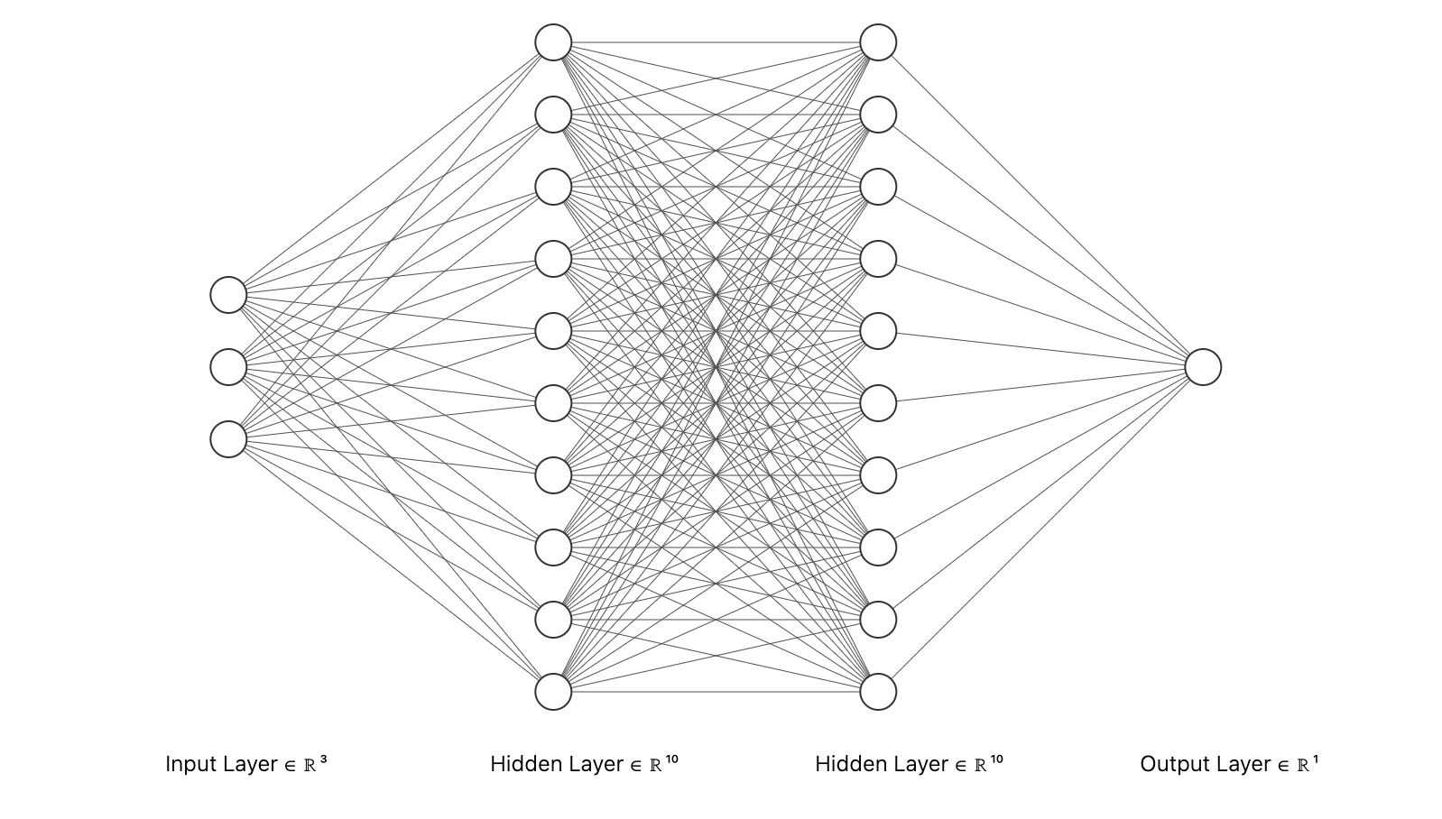 MLP with input layer with 3 nodes, 2 hidden layers with 10 nodes each, and an output layer with 1 node - Image by Author
Multi-Layer Perceptrons (MLPs) are a core component of modern neural networks. They consist of layers of interconnected nodes, or "neurons," designed to approximate complex, non-linear functions by learning from data. Each neuron uses a fixed activation function on the weighted sum of its inputs, transforming input data into the desired output through multiple layers of abstraction. MLPs have driven breakthroughs in various fields, from computer vision to speech recognition.
However, MLPs have some significant limitations:
- Fixed Activation Functions on Nodes : Each node in an MLP has a predetermined activation function, like ReLU or Sigmoid. While effective in many cases, these fixed functions limit the network's flexibility and adaptability. This can make it challenging for MLPs to optimize certain types of functions or adapt to specific data characteristics.
- Interpretability Issues : MLPs are often criticized for being "black boxes." As they become more complex, understanding their decision-making process becomes harder. The fixed activation functions and intricate weight matrices obscure the network's inner workings, making it difficult to interpret and trust the model's predictions without extensive analysis.
These drawbacks highlight the need for alternatives that offer greater flexibility and interpretability, paving the way for innovations like Kolmogorov-Arnold Networks (KANs).
2: Kolmogorov-Arnold Networks (KANs)
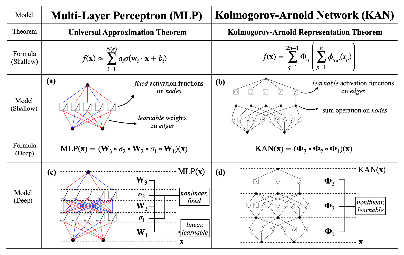 MLP vs KAN comparison -Imake by Kan Github Repo (License)
The Kolmogorov-Arnold representation theorem, formulated by mathematicians Andrey Kolmogorov and Vladimir Arnold, states that any multivariate continuous function can be represented as a finite composition of continuous functions of a single variable and the operation of addition. Think of this theorem as breaking down a complex recipe into individual, simple steps that anyone can follow. Instead of dealing with the entire recipe at once, you handle each step separately, making the overall process more manageable. This theorem implies that complex, high-dimensional functions can be broken down into simpler, univariate functions.
For neural networks, this insight is revolutionary, it suggests that a network could be designed to learn these univariate functions and their compositions, potentially improving both accuracy and interpretability.
KANs leverage the power of the Kolmogorov-Arnold theorem by fundamentally altering the structure of neural networks. Unlike traditional MLPs, where fixed activation functions are applied at each node, KANs place learnable activation functions on the edges (weights) of the network. This key difference means that instead of having a static set of activation functions, KANs adaptively learn the best functions to apply during training. Each edge in a KAN represents a univariate function parameterized as a spline, allowing for dynamic and fine-grained adjustments based on the data.
This change enhances the network's flexibility and ability to capture complex patterns in data, providing a more interpretable and powerful alternative to traditional MLPs. By focusing on learnable activation functions on edges, KANs effectively utilize the Kolmogorov-Arnold theorem to transform neural network design, leading to improved performance in various AI tasks.
3: Mathematical Foundations
At the core of Kolmogorov-Arnold Networks (KANs) is a set of equations that define how these networks process and transform input data. The foundation of KANs lies in the Kolmogorov-Arnold representation theorem, which inspires the structure and learning process of the network.
Imagine you have an input vector x=[x1,x2,...,xn], which represents data points that you want to process. Think of this input vector as a list of ingredients for a recipe.
The theorem states that any complex recipe (high-dimensional function) can be broken down into simpler steps (univariate functions). For KANs, each ingredient (input value) is transformed through a series of simple steps (univariate functions) placed on the edges of the network. Mathematically, this can be represented as:
 KAN Formula - Image by Author
Here, ϕ_q,p are univariate functions that are learned during training. Think of ϕ_q,p as individual cooking techniques for each ingredient, and Φ_q as the final assembly step that combines these prepared ingredients.
Each layer of a KAN applies these cooking techniques to transform the ingredients further. For layer l, the transformation is given by:
 Kan Layer Transformation Formula - Image by Author
Here, x(l) denotes the transformed ingredients at layer l, and ϕ_l,i,j are the learnable univariate functions on the edges between layer l and l+1. Think of this as applying different cooking techniques to the ingredients at each step to get intermediate dishes.
The output of a KAN is a composition of these layer transformations. Just as you would combine intermediate dishes to create a final meal, KANs combine the transformations to produce the final output:
 KAN Output Formula - Image by Author
Here, Φl represents the matrix of univariate functions at layer l. The overall function of the KAN is a composition of these layers, each refining the transformation further.
MLPs Structure In traditional MLPs, each node applies a fixed activation function (like ReLU or sigmoid) to its inputs. Think of this as using the same cooking technique for all ingredients, regardless of their nature.
MLPs use linear transformations followed by these fixed non-linear activations:
 MLP Formula - Image by Author
where W represents the weight matrices, and σ represents the fixed activation functions.
Grid Extension Technique
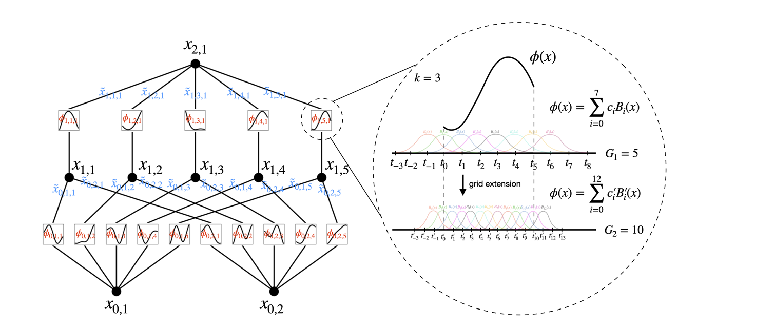 Left: Notations of activations that flow through the network. Right: an activation function is parameterized as a B-spline, which allows switching between coarse-grained and fine-grained grids - Imagine extracted by "KAN: Kolmogorov-Arnold Networks" (License)
Grid extension is a powerful technique used to improve the accuracy of Kolmogorov-Arnold Networks (KANs) by refining the spline grids on which the univariate functions are defined. This process allows the network to learn increasingly detailed patterns in the data without requiring complete retraining.
These B-splines are a series of polynomial functions that are pieced together to form a smooth curve. They are used in KANs to represent the univariate functions on the edges. The spline is defined over a series of intervals called grid points. The more grid points there are, the finer the detail that the spline can capture
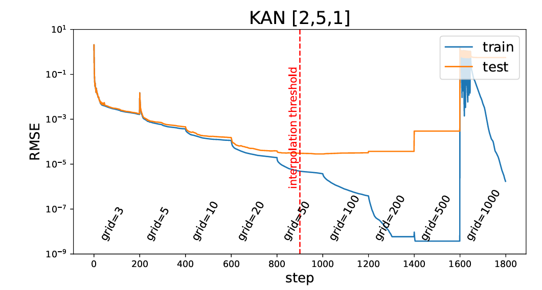 KAN with 2D input, 1 hidden layer with 5 nodes, and an output layer with 1 node - Imagine extracted by "KAN: Kolmogorov-Arnold Networks" (License)
Initially, the network starts with a coarse grid, which means there are fewer intervals between grid points. This allows the network to learn the basic structure of the data without getting bogged down in details. Think of this like sketching a rough outline before filling in the fine details.
As training progresses, the number of grid points is gradually increased. This process is known as grid refinement. By adding more grid points, the spline becomes more detailed and can capture finer patterns in the data. This is similar to progressively adding more detail to your initial sketch, turning it into a detailed drawing.
Each increase introduces new B-spline basis functions B′_m(x). The coefficients c'_m for these new basis functions are adjusted to ensure that the new, finer spline closely matches the original, coarser spline.
To achieve this match, least squares optimization is used. This method adjusts the coefficients c'_m to minimize the difference between the original spline and the refined spline.
 Least Square Optimization Formula - Image by Author
Essentially, this process ensures that the refined spline continues to accurately represent the data patterns learned by the coarse spline.
Simplification Techniques
To enhance the interpretability of KANs, several simplification techniques can be employed, making the network easier to understand and visualize.
Sparsification and Pruning This technique involves adding a penalty to the loss function based on the L1 norm of the activation functions. The L1 norm for a function ϕ is defined as the average magnitude of the function across all input samples:
 L1 Norm Formula - Image by Author
Here, N_p is the number of input samples, and ϕ(x_s) represents the value of the function ϕ for the input sample x_s.
Think of sparsification like decluttering a room. By removing unnecessary items (or reducing the influence of less important functions), you make the space (or network) more organized and easier to navigate.
After applying L1 regularization, the L1 norms of the activation functions are evaluated. Neurons and edges with norms below a certain threshold are considered insignificant and are pruned away. The threshold for pruning is a hyperparameter that determines how aggressive the pruning should be.
Pruning is like trimming a tree. By cutting away the weak and unnecessary branches, you allow the tree to focus its resources on the stronger, more vital parts, leading to a healthier and more manageable structure.
Symbolification Another approach is to replace learned univariate functions with known symbolic forms to make the network more interpretable.
The task is to identify potential symbolic forms (e.g., sin, exp) that can approximate the learned functions. This step involves analyzing the learned functions and suggesting symbolic candidates based on their shape and behavior.
Once symbolic candidates are identified, use grid search and linear regression to fit parameters such that the symbolic function closely approximates the learned function.
4: KAN vs MLP in Python
To demonstrate the capabilities of Kolmogorov-Arnold Networks (KANs) compared to traditional Multi-Layer Perceptrons (MLPs), we will fit a function-generated dataset to both a KAN model and MLP model (leveraging PyTorch), to see what their performances look like.
The function we will be using is the same one used by the authors of the paper to show KAN's capabilities vs MLP (Original paper example). However, the code will be different. You can find all the code we will cover today in this Notebook:
models-from-scratch-python/KAN - Kolmogorov-Arnold Networks/demo.ipynb at main ·...
Let's import the required libraries, and generate the dataset
javascript
import numpy as np
import torch
import torch.nn as nn
from torchsummary import summary
from kan import KAN, create_dataset
import matplotlib.pyplot as plt
Here, we use:
numpy: For numerical operations.torch: For PyTorch, which is used for building and training neural networks.torch.nn: For neural network modules in PyTorch.torchsummary: For summarizing the model structure.kan: Custom library containing the KAN model and dataset creation functions.matplotlib.pyplot: For plotting and visualizations.
python
# Define the dataset generation function
f = lambda x: torch.exp(torch.sin(torch.pi * x[:, [0]]) + x[:, [1]] ** 2)
This function includes both sinusoidal (sin) and exponential (exp) components. It takes a 2D input x and computes the output using the formula:
 Dataset generation Function - Image by Author
Let's now fit a tensor of 100 points uniformly distributed between [-2, 2] to this function, to see what it looks like:
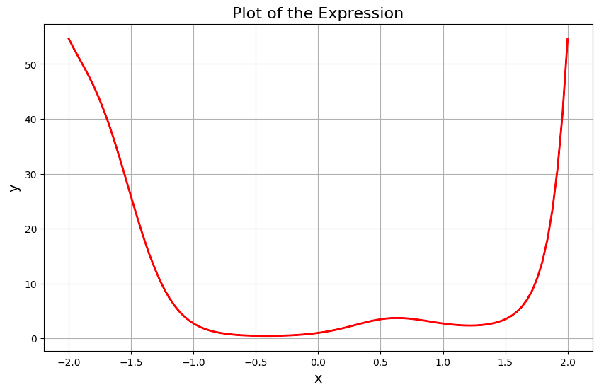 Plot generated by fitting 100 points uniformly distributed between [-2, 2] to Dataset generation function - Image by Author
python
# Create the dataset
dataset = create_dataset(f, n_var=2)
create_dataset generates a dataset based on the function f. The dataset includes input-output pairs that will be used for training and testing the neural networks.
Now let's build a KAN model and train it on the dataset. We will start with a coarse grid (5 points) and gradually refine it (up to 100 points). This improves the model's accuracy by capturing finer details in the data.
python
grids = np.array([5, 10, 20, 50, 100])
train_losses_kan = []
test_losses_kan = []
steps = 50
k = 3

for i in range(grids.shape[0]):
    if i == 0:
        model = KAN(width=[2, 1, 1], grid=grids[i], k=k)
    else:
        model = KAN(width=[2, 1, 1], grid=grids[i], k=k).initialize_from_another_model(model, dataset['train_input'])
    results = model.train(dataset, opt="LBFGS", steps=steps, stop_grid_update_step=30)
    train_losses_kan += results['train_loss']
    test_losses_kan += results['test_loss']

    print(f"Train RMSE: {results['train_loss'][-1]:.8f} | Test RMSE: {results['test_loss'][-1]:.8f}")
In this example, we define an array called grids with values [5, 10, 20, 50, 100]. We iterate over these grids to fit models sequentially, meaning each new model is initialized using the previous one.
For each iteration, we define a model with k=3, where k is the order of the B-spline. We set the number of training steps (or epochs) to 50. The model's architecture consists of an input layer with 2 nodes, one hidden layer with 1 node, and an output layer with 1 node. We use the LFGBS optimizer for training.
Here are the training and test losses during the training process:
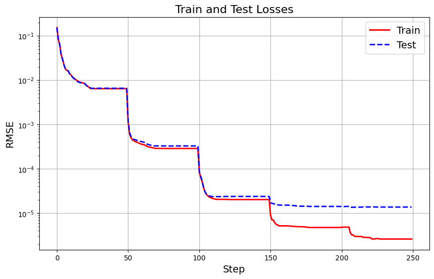 KAN Train and Test Losses Plot - Image by Author
Let's now define and train a traditional MLP for comparison.
python
# Define the MLP
class MLP(nn.Module):
    def __init__(self):
        super(MLP, self).__init__()
        self.layers = nn.Sequential(
            nn.Linear(dataset['train_input'].shape[1], 64),
            nn.ReLU(),
            nn.Linear(64, 64),
            nn.ReLU(),
            nn.Linear(64, 1)
        )
    def forward(self, x):
        return self.layers(x)

# Instantiate the model
model = MLP()
summary(model, input_size=(dataset['train_input'].shape[1],))
The MLP has an input layer, two hidden layers with 64 neurons each, and an output layer. ReLU activation is used between the layers.
python
criterion = nn.MSELoss()
optimizer = torch.optim.Adam(model.parameters(), lr=1e-2)
train_loss_mlp = []
test_loss_mlp = []

epochs = 250
for epoch in range(epochs):
    optimizer.zero_grad()
    output = model(dataset['train_input']).squeeze()
    loss = criterion(output, dataset['train_label'])
    loss.backward()
    optimizer.step()
    train_loss_mlp.append(loss.item()**0.5)

    # Test the model
    model.eval()
    with torch.no_grad():
        output = model(dataset['test_input']).squeeze()
        loss = criterion(output, dataset['test_label'])
        test_loss_mlp.append(loss.item()**0.5)

    print(f'Epoch {epoch+1}/{epochs}, Train Loss: {train_loss_mlp[-1]:.2f}, Test Loss: {test_loss_mlp[-1]:.2f}', end='r')
We use mean squared error (MSE) loss and Adam optimizer, and train the model for 250 epochs, recording the training and testing losses.
This is what the train and test RMSE look like in MLP:
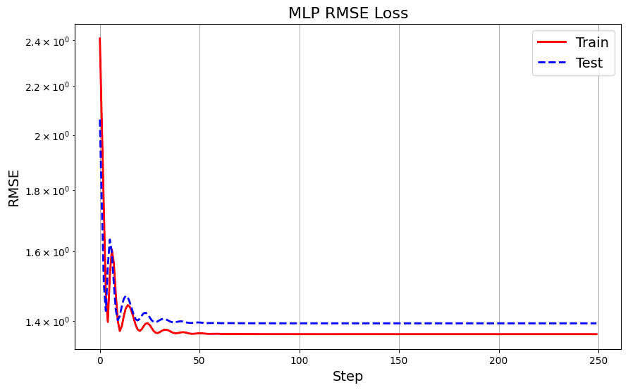 MLP Train and Test Losses Plot - Image by Author
Let's put side to side the loss plots for a comparison:
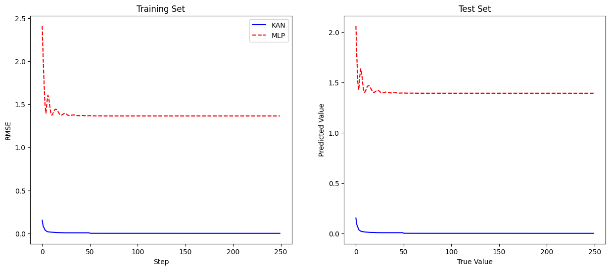 KAN vs MLP training losses plot (left) and test losses plot (right) - Image by Author
The plot shows that the KAN model achieves lower training RMSE than the MLP model, indicating better function-fitting capability. Similarly, the KAN model outperforms the MLP on the test set, demonstrating its superior generalization ability.
This example illustrates how KANs can more accurately fit complex functions than traditional MLPs, thanks to their flexible and adaptive structure. By refining the grid and employing learnable univariate functions on the edges, KANs capture intricate patterns in the data that MLPs may miss, leading to improved performance in function-fitting tasks.
Does this mean we should switch to KAN models permanently? Not necessarily.
KANs showed great results in this example, but when I tested them on other scenarios with real data, MLPs often performed better. One thing you'll notice when working with KAN models is their sensitivity to hyperparameter optimization. Also, KANs have primarily been tested using spline functions, which work well for smoothly varying data like our example but might not perform as well in other situations.
In summary, KANs are definitely intriguing and have a lot of potential, but they need more study, especially regarding different datasets and the algorithm's inner workings, to really make them work effectively.
5: Advantages of KANs
Accuracy
One of the standout advantages of Kolmogorov-Arnold Networks (KANs) is their ability to achieve higher accuracy with fewer parameters compared to traditional Multi-Layer Perceptrons (MLPs). This is primarily due to the learnable activation functions on the edges, which allow KANs to better capture complex patterns and relationships in the data.
Unlike MLPs that use fixed activation functions at each node, KANs use univariate functions on the edges, making the network more flexible and capable of fine-tuning its learning process to the data.
Because KANs can adjust the functions between layers dynamically, they can achieve comparable or even superior accuracy with a smaller number of parameters. This efficiency is particularly beneficial for tasks with limited data or computational resources.
Interpretability
KANs offer significant improvements in interpretability over traditional MLPs. This enhanced interpretability is crucial for applications where understanding the decision-making process is as important as the outcome.
KANs can be simplified through techniques like sparsification and pruning, which remove unnecessary functions and parameters. These techniques not only improve interpretability but also enhance the network's performance by focusing on the most relevant components.
For some functions, it is possible to identify symbolic forms of the activation functions, making it easier to understand the mathematical transformations within the network.
Scalability
KANs exhibit faster neural scaling laws compared to MLPs, meaning they improve more rapidly as the number of parameters increases.
KANs benefit from more favorable scaling laws due to their ability to decompose complex functions into simpler, univariate functions. This allows them to achieve lower error rates with increasing model complexity more efficiently than MLPs.
KANs can start with a coarser grid and extend it to finer grids during training, which helps in balancing computational efficiency and accuracy. This approach allows KANs to scale up more gracefully than MLPs, which often require complete retraining when increasing model size.
Conclusion
Kolmogorov-Arnold Networks (KANs) present a groundbreaking alternative to traditional Multi-Layer Perceptrons (MLPs), offering several key innovations that address the limitations of their predecessors. By leveraging learnable activation functions on the edges rather than fixed functions at the nodes, KANs introduce a new level of flexibility and adaptability. This structural change leads to:
- Enhanced Accuracy : KANs achieve higher accuracy with fewer parameters, making them more efficient and effective for a wide range of tasks.
- Improved Interpretability : The ability to visualize and simplify KANs aids in understanding the decision-making process, which is crucial for critical applications in healthcare, finance, and autonomous systems.
- Better Scalability : KANs exhibit faster neural scaling laws, allowing them to handle increasing complexity more gracefully than MLPs.
The introduction of Kolmogorov-Arnold Networks marks an exciting development in the field of neural networks, opening up new possibilities for AI and machine learning.
References
Register Now to Continue Reading
Unlock Towards Data Science with a Free Account
All articles on Towards Data Science are available to registered users. Create a free account today to access this article and thousands more.
Register for freeSign in to your account
 Written By
See all from Cristian Leo
Data ScienceMachine LearningMathematicsProgrammingThoughts And Theory
Share This Article
Towards Data Science is a community publication. Submit your insights to reach our global audience and earn through the TDS Author Payment Program.
Write for TDS
Related Articles
Machine Learning
How to teach an intelligent agent to play simple games using State-Action-Reward-State-Action (SARSA) algorithm
Saul Dobilas
October 20, 202213 min read
Artificial Intelligence
How to Create a Searchable Archive of PDFs with OCR, Python, & SQLite
Brandon Cosley
August 10, 20219 min read
Artificial Intelligence
Learn how to create new columns in Spark data frames
Soner Yıldırım
December 20, 20214 min read
Machine Learning
It's about Data, Skills, Tools...and especially Culture!
Col Jung
July 19, 202316 min read
Machine Learning
Uncovering a simple yet powerful, award-winning machine learning algorithm
Gurjinder Kaur
November 12, 20249 min read
Artificial Intelligence
A closer look at understanding why the Sum of Squares is important to Data Science
Mike Wolfe
June 14, 20225 min read
Programming
Ten easy ways to sort data in pandas
Parul Pandey
March 22, 20217 min read
Machine Learning
I paid a visit to this museum about four months ago on a tour of Wellington, the windiest capital of the world. The Maori name, 'Te Papa...
Herman Wandabwa
July 22, 20192 min read
Deep Learning
Data can be deceptive, so be on your toes!
Michael Clayton
August 16, 202410 min read
Your home for data science and AI. The world's leading publication for data science, data analytics, data engineering, machine learning, and artificial intelligence professionals.
Subscribe to Our NewsletterWrite For TDS•About•Advertise•Privacy Policy•Terms of Use
© Insight Media Group, LLC 2026•The New Stack•roadmap.sh•Creator Network
Recommended Articles
Close