Last time, right at the end, I asked a question and then walked away from it. Will this order be late, or won't it? The final answer isn't a number on a continuous scale. It's a class: yes or no.
Every model we've built so far in this series has answered a different kind of question — how many minutes, how much rent, how many rupees. All numbers that can sit anywhere on a scale.
"Will it be late" doesn't have a continuous answer like that. The final class is either yes or no. But as we'll see, the model can still use a number to express how likely each class is.
So here's what I want to do in this post: take the model we already trust, the straight line, and try it on this new kind of question. Not because I expect it to work. Because watching it fail, and seeing exactly how it fails, is the fastest way to understand why we need something new.
Go back to the delivery orders we've been using this whole series. Distance from the restaurant, and how long the order actually took.
| Distance (km) | Time Taken (min) |
|---|---|
| 1 | 14 |
| 3 | 22 |
| 5 | 30 |
| 7 | 41 |
| 9 | 47 |
| 11 | 55 |
"Predict the time" is a regression question. That's what we've been doing since the first post. Give the model a distance, get back a number of minutes.
Now let's ask something else about these exact same orders. Say anything over 40 minutes counts as late. Look at the same table again, but this time with a late column added.
| Distance (km) | Time Taken (min) | Late? |
|---|---|---|
| 1 | 14 | No |
| 3 | 22 | No |
| 5 | 30 | No |
| 7 | 41 | Yes |
| 9 | 47 | Yes |
| 11 | 55 | Yes |
Same orders. Same distances. Completely different question. "How long will it take" wants a number. "Will it be late" wants a decision. One output is continuous, it can be 14.2 minutes or 39.9 minutes, anything at all. The other output only ever has two possible values. Late, or not late. There's nothing in between.
One honest note before we go further: this little dataset is unusually clean. Every short order comes back not late, every long order comes back late, no exceptions. Real delivery data wouldn't be this polite — two orders at the same distance could land on opposite sides because of traffic, a slow kitchen, or a bad light. I'm keeping it this clean on purpose, because right now I want to isolate one problem: why a straight line makes a bad probability model. Messier data can come later.
That difference sounds small when you write it in a sentence. It is not small to a model.
Here's the thing about "no" and "yes." A computer doesn't understand words like that. So before we can do anything, we turn them into numbers. No becomes 0. Yes becomes 1.
| Distance (km) | Late (0 = No, 1 = Yes) |
|---|---|
| 1 | 0 |
| 3 | 0 |
| 5 | 0 |
| 7 | 1 |
| 9 | 1 |
| 11 | 1 |
Now look at that table honestly for a second. It's still a distance column and a number column. Nothing about it looks different from any of the tables we've fit a straight line to before. So why not just do exactly that? Feed it into the same gradient descent code, and see what happens.
w, b = gradient_descent(distances, late, learning_rate=0.01, iterations=20000)
print(w, b)
w: 0.1286
b: -0.2714
Nothing exploded. No error. The model trained just fine — it found a line that minimizes the same squared-error cost we've been using this whole series. Let's look at what it predicts for each order.
| Distance | Actual (0 or 1) | Line's Prediction |
|---|---|---|
| 1 | 0 | −0.143 |
| 3 | 0 | 0.114 |
| 5 | 0 | 0.371 |
| 7 | 1 | 0.629 |
| 9 | 1 | 0.886 |
| 11 | 1 | 1.143 |
Before trusting that table, let's check one row by hand, the way we've done in earlier posts. Take the order at 7 km:
 prediction = 0.1286(7) - 0.2714
 prediction = 0.9002 - 0.2714
 prediction = 0.6288
The actual label is 1. The line gives us 0.629. If we pretend that number is a probability, that's about 63% — not a crazy number on its own. And that's the tricky part: 0.629 looks perfectly reasonable as a probability, but looking reasonable isn't the same as actually being one. The trouble shows up at the edges.
Stop on that first row for a second. The actual answer is 0. Not "close to zero." Just zero, flat, that's the whole answer. And the line predicts −0.143.
We could try to read that as a probability, but that's exactly where things fall apart. What does negative 0.143 mean here? Negative fourteen percent chance of being late? There's no such thing as a negative chance. You can't be less than 0% sure of anything. The number the line gave us doesn't correspond to any real answer in the world.
Now look at the last row. Actual answer is 1. The line predicts 1.143 — treat that as a probability and it's saying 114.3% chance of being late. That's not just wrong, it's wrong in a way that shouldn't even be possible. The model has somehow become more than certain. Certainty tops out at 100%.
My first instinct, the first time I saw this, was to think: fine, just round it. Anything below 0.5 becomes "not late," anything above becomes "late." Problem solved, right?
Worth pausing on that 0.5 for a second — it isn't something the model learned. It's a threshold we chose, a rule for turning a continuous number into a yes-or-no decision. It'll matter a lot more once we get to the next model.
Rounding does patch the output. But it doesn't fix what's actually broken. Try feeding the model a distance a bit further out than anything it saw during training.
for d in [13, 15]:
    print(d, w*d + b)
13  1.4
15  1.657
At 15 km, the line is telling us the order is 165.7% likely to be late. Rounding will happily turn that into "late," and get the direction right. But it's getting the right answer by accident, using a number that never meant anything in the first place.
And here's the part that actually matters. This isn't a bug we can fix by tweaking the learning rate, training longer, or picking a better starting point — it's baked into what a straight line is. A line has no ceiling and no floor. Give it enough distance in either direction, and it will keep climbing or keep falling, forever. That's just what a line is.
But "chance of being late" isn't allowed to do that. It has a hard floor at 0 and a hard ceiling at 1, because that's what probability means. Zero percent is the least sure you can ever be. A hundred percent is the most. A tool that can't stay inside those two walls was never going to be the right tool for a question shaped like this one.
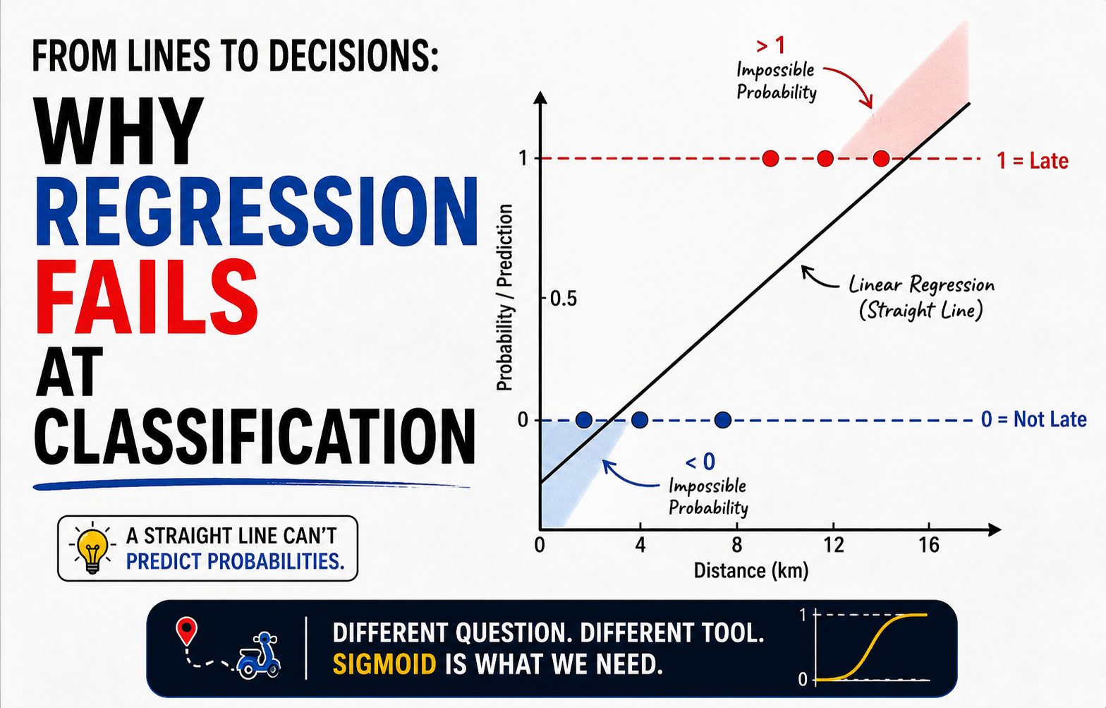
Picture the six points from our table plotted out. Three sitting flat on the 0 line for the shorter distances. Three sitting flat on the 1 line for the longer ones. Somewhere in between, a jump.
Now picture our straight line drawn through that same plot. It slides up gently, left to right, the way every line we've trained in this series has. On the left side of the picture, it dips below the 0 line, into negative numbers. On the right side, it rises above the 1 line, into numbers bigger than one.
That's the whole problem, in one image. The data lives strictly between two flat walls, 0 and 1. The line doesn't know those walls exist. Nobody told it. We only ever taught it to minimize error, we never taught it that probabilities have limits. So it does what it's always done, follow the slope, and walk straight through the walls like they aren't there.
So here's where we've landed. Regression is the right tool when you're trying to predict a continuous quantity. Delivery time, rent, mileage, whatever. But the moment we want the model to estimate the probability of one class or another, a plain straight line stops making sense. It has no way to respect the floor at 0 or the ceiling at 1, because nothing about it was ever built to have floors or ceilings in the first place.
What we actually need is something that behaves like a line everywhere in the middle, but bends and flattens out the moment it gets close to 0 or close to 1. Something that can climb, but never quite touches the ceiling. Something that can fall, but never quite touches the floor.
That shape has a name, and it's one of the most useful little curves in all of machine learning. It's called the sigmoid function, and it's exactly what we're building next.
The full code for this post is up on GitHub here: https://github.com/tharun-pandya/Machine-Learning-Blog-Series/blob/main/Regression_Fails_At_Classification.ipynb
See you in the next one.