Do Bigger GPT Models Always Perform Better?

TL;DR: What I tested and observed

• Experiment 1 — Different sizes, fixed tokens: I increased model width, depth, and total parameter count while giving every model the same 200,192 training tokens. In this setup, the smallest model achieved the lowest validation loss and trained the fastest.

• Experiment 2 — Width versus depth: I kept the total parameter count close to 13.3 million but distributed those parameters differently. The wider, shallower model produced the best validation result and substantially higher throughput than the deeper alternatives.

• Experiment 3 — Fixed estimated compute: I gave smaller models more training tokens and larger models fewer so that estimated training compute remained approximately equal. In this comparison, the smallest model achieved the strongest result by a relatively large margin.

GitHub: View the complete experiment notebook

These results do not tell us that smaller or shallower models are universally better. They show what happened with this particular model architecture, WikiText dataset, hardware, and limited training budget.

---

When we hear that a model has more parameters, it is natural to assume that it should perform better.

More parameters give a model additional capacity. In theory, that capacity can help it represent more complex patterns and relationships. But a larger model may also need more data, optimization steps, and compute before that additional capacity becomes useful.

Research on scaling laws has explored how model size, training data, and compute interact. Other studies have asked whether parameter count alone is enough to describe a model—or whether the way those parameters are distributed across width and depth also matters.

I used these ideas as inspiration and explored the same questions using the small GPT-style model and WikiText dataset from my previous experiments:

Given my model architecture, dataset, hardware, and training budget, what happens when I change model capacity and how that capacity is distributed?

---

Experiment 1: Increasing overall model capacity

For the first experiment, I created three progressively larger models:

CAPACITY_TOKEN_BUDGET = 200_000

CAPACITY_CONFIGS = [
    {"label": "small",    "emb_dim": 64,  "n_heads": 2, "n_layers": 2},
    {"label": "baseline", "emb_dim": 128, "n_heads": 4, "n_layers": 4},
    {"label": "large",    "emb_dim": 192, "n_heads": 6, "n_layers": 6},
]

Model	Embedding dimension	Attention heads	Transformer blocks	Parameters
Small	64	2	2	6.54M
Baseline	128	4	4	13.67M
Large	192	6	6	21.99M

The embedding dimension, attention-head count, number of transformer blocks, and total parameter count increased together.

Every model processed the same 200,192 training tokens over 782 optimizer steps.

This was a fixed-token comparison: each model saw the same amount of training data, but the larger models performed more computation for every token.

My hypothesis

I expected the larger models to achieve lower validation loss because they had more representational capacity.

At the same time, I expected the improvement to diminish as the models became larger, especially because all three received the same relatively small token budget.

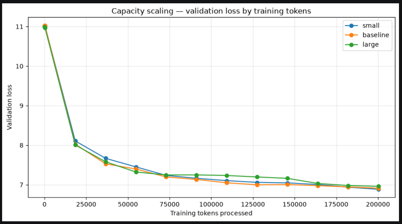
The results did not follow that pattern.

Results

Metric	Small	Baseline	Large
Embedding dimension	64	128	192
Attention heads	2	4	6
Transformer blocks	2	4	6
Parameters	6.54M	13.67M	21.99M
Training tokens	200,192	200,192	200,192
Runtime	146.7 sec	239.9 sec	388.3 sec
Tokens per second	1,364.7	834.3	515.6
Peak memory	714.9 MB	854.0 MB	990.7 MB
Final validation loss ↓	6.8850	6.9119	6.9598
Perplexity ↓	977.46	1,004.12	1,053.45
Top-1 accuracy ↑	12.19%	12.58%	11.48%
Estimated compute	0.0079 PFLOPs	0.0164 PFLOPs	0.0264 PFLOPs

In this run, the smallest model achieved the lowest validation loss and perplexity.

The baseline model produced slightly higher top-1 accuracy, although the difference was only 0.39 percentage points. Its validation loss was still higher than the small model’s.

Accuracy and cross-entropy loss measure different things. Accuracy only checks whether the model’s highest-scoring token was correct. Loss also considers how much probability the model assigned to the correct token.

The large model was worse on both validation loss and top-1 accuracy.

What changed as the model became larger?

Moving from the small model to the large model:

• Parameter count increased from 6.54 million to 21.99 million.

• Runtime increased from 146.7 to 388.3 seconds.

• Throughput fell from 1,364.7 to 515.6 tokens per second.

• Peak memory increased from 714.9 MB to 990.7 MB.

• Validation loss increased from 6.8850 to 6.9598.

In this setup, increasing capacity increased the cost of training without improving the final validation result.

One possible interpretation is that the larger models were undertrained relative to their capacity. They had more parameters to optimize but received exactly the same number of training tokens and optimizer steps as the smaller model.

This does not mean that the larger models could never perform better. They may have needed more training tokens, additional optimizer steps, a different learning rate, different regularization, or a larger and more varied dataset.

The result only tells us that the additional capacity did not help under the conditions used in this experiment.

The fixed-token comparison answers:

Which model performed better after seeing the same amount of training data?

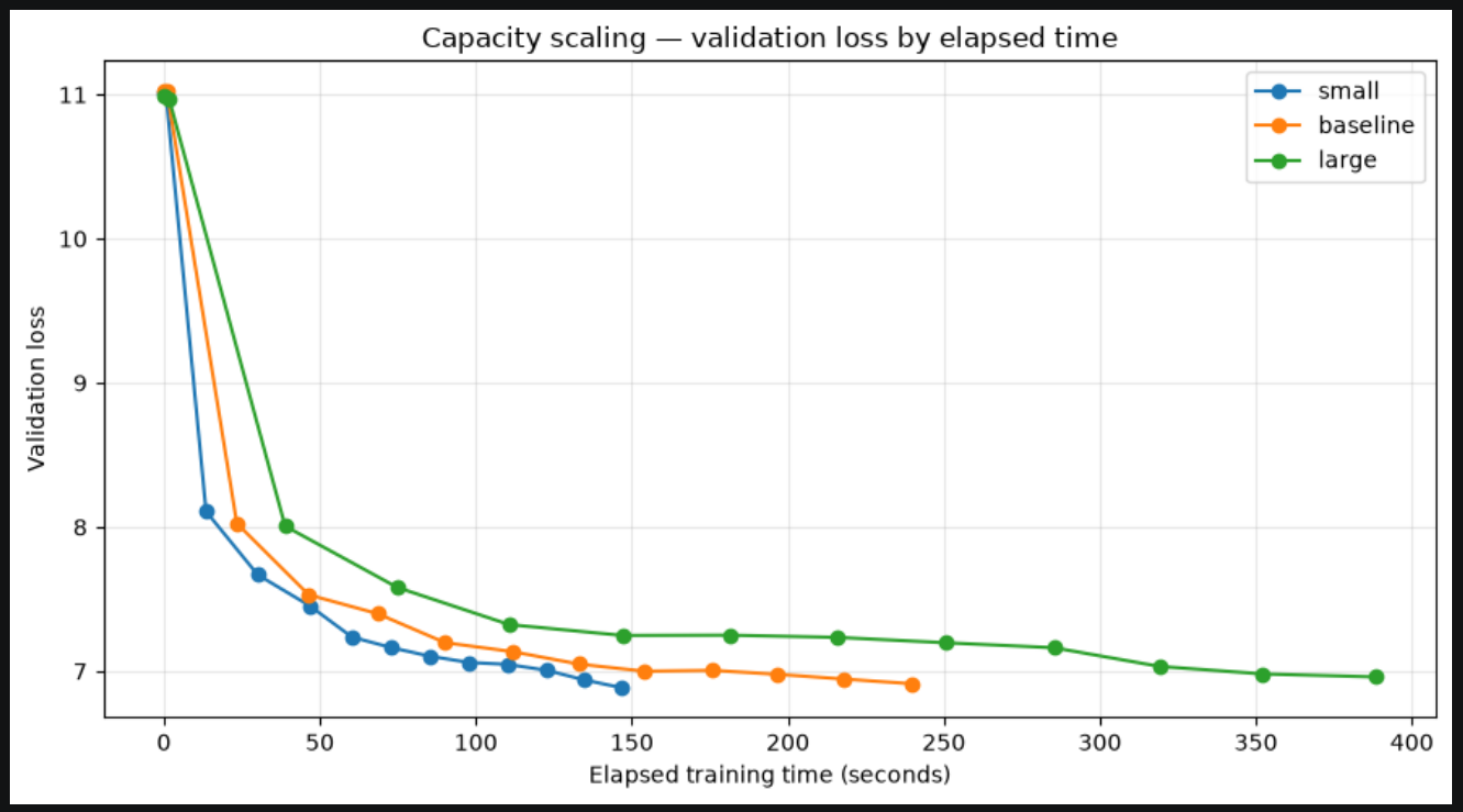
I also evaluated the models under a fixed wall-clock budget. As expected, the smaller model processed more tokens and returned a lower validation loss than the larger models.

---

Experiment 2: Where should the parameters go?

Experiment 1 changed several architectural variables together. The larger models were wider, deeper, and larger in total parameter count.

That made it difficult to know whether the result was mainly related to overall capacity, additional depth, or a combination of both.

For the second experiment, I kept the total parameter count nearly constant and changed how that capacity was distributed:

SHAPE_TOKEN_BUDGET = 200_000

SHAPE_CONFIGS = [
    {"label": "wide_shallow", "emb_dim": 128, "n_heads": 4, "n_layers": 2},
    {"label": "balanced",     "emb_dim": 120, "n_heads": 4, "n_layers": 7},
    {"label": "narrow_deep",  "emb_dim": 112, "n_heads": 4, "n_layers": 13},
]

Shape	Embedding dimension	Attention heads	Transformer blocks	Parameters
Wide–shallow	128	4	2	13.28M
Balanced	120	4	7	13.29M
Narrow–deep	112	4	13	13.24M

The parameter spread across the three models was less than 0.4%, with each model containing approximately 13.3 million parameters.

My hypothesis

I thought the deeper model might learn richer transformations by applying more transformer blocks sequentially.

At the same time, I expected it to train more slowly because those blocks must execute one after another. This could have created a quality-versus-speed trade-off.

That trade-off did not appear in my results.

Fixed-token results

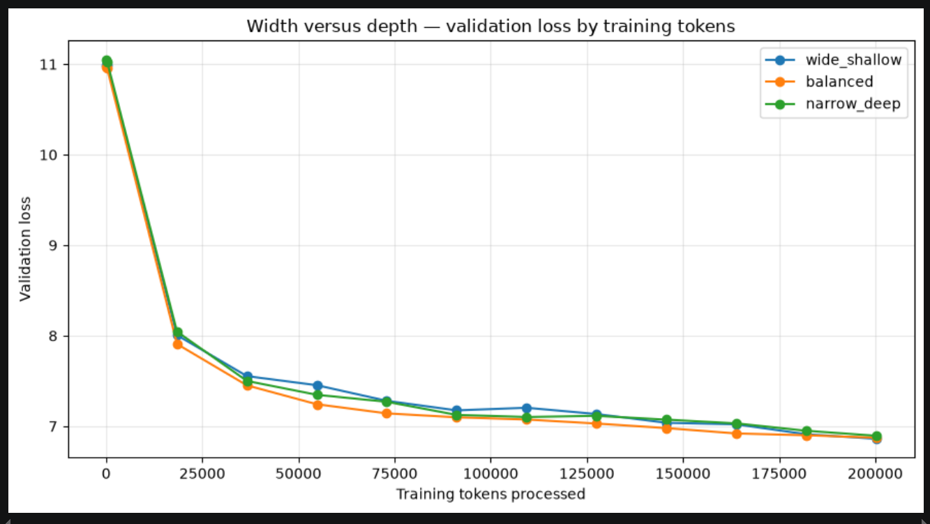
Metric	Wide–shallow	Balanced	Narrow–deep
Embedding dimension	128	120	112
Attention heads	4	4	4
Transformer blocks	2	7	13
Parameters	13.28M	13.29M	13.24M
Training tokens	200,192	200,192	200,192
Runtime	208.0 sec	296.0 sec	367.7 sec
Tokens per second	962.6	676.2	544.5
Peak memory	903.4 MB	946.7 MB	846.9 MB
Final validation loss ↓	6.8615	6.8739	6.8949
Perplexity ↓	954.77	966.73	987.26
Top-1 accuracy ↑	13.05%	11.80%	12.03%
Estimated compute	0.0159 PFLOPs	0.0160 PFLOPs	0.0159 PFLOPs

Compared with the narrow–deep model, the wide–shallow model:

• Completed the run approximately 44% faster.

• Processed about 77% more tokens per second.

• Achieved validation loss that was 0.0334 lower.

• Achieved top-1 accuracy that was approximately one percentage point higher.

Despite having similar parameter counts and estimated compute, the three models had very different runtimes.

A deeper model must execute more transformer blocks sequentially. In this setup, that additional depth increased runtime without producing an obvious quality benefit.

The absolute loss difference was not enormous, so I would not interpret this as a universal preference for shallow models.

What stood out more clearly was that the deeper architecture did not show enough improvement to compensate for its substantially longer runtime.

---

Experiment 3: Same estimated compute, different allocations

In Experiment 1, every model processed the same number of tokens. This meant that the larger models also consumed more estimated computation.

For the final experiment, I held approximate training compute constant instead.

I used the following approximation:

$$C \approx 6NT$$

where:

• (C) is estimated training compute.

• (N) is the number of model parameters.

• (T) is the number of training tokens.

Under this approximation, a model with more parameters must process fewer tokens if the overall compute budget remains fixed.

The resulting configurations were:

Model	Parameters	Token budget	Estimated compute
Small	6.54M	418,304	0.0164 PFLOPs
Baseline	13.67M	200,192	0.0164 PFLOPs
Large	21.99M	124,416	0.0164 PFLOPs

Based on the first experiment, I expected the small model to benefit from receiving more training tokens.

But I did not know whether that advantage would be large enough to overcome the additional representational capacity of the larger models.

The result was much clearer than in the earlier comparisons.

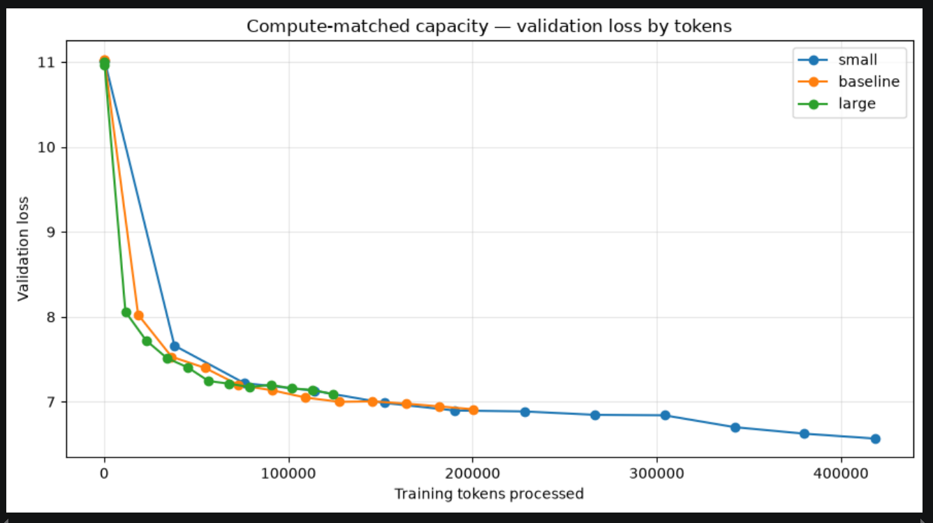
The smallest model achieved the strongest result by the largest margin of the three experiments.

One possible interpretation is that, under this estimated compute budget, the small model benefited more from additional training exposure than the large model benefited from additional capacity.

The large model had more parameters, but it received only 124,416 training tokens. In this setup, that may not have been enough training for the model to use its additional capacity effectively.

---

What I observed across the three experiments

Each experiment answered a slightly different question.

Fixed tokens

The smallest model achieved the lowest validation loss among the progressively scaled small, baseline, and large configurations.

The larger models required more runtime, memory, and estimated compute, but the additional capacity did not improve validation quality within the 200,192-token budget.

Approximately fixed parameter count

The wide–shallow architecture achieved the best validation result and the highest training throughput.

The deeper architectures did not show enough quality improvement to compensate for their additional runtime. In these runs, their validation results were also slightly worse.

Fixed estimated compute

The smallest model processed substantially more training tokens and achieved the strongest result by the largest margin.

In this setup, allocating the budget toward more training exposure appeared more effective than allocating it toward a larger parameter count.

---

Limitations of the experiment

One learning rate for every architecture

One primary random seed

Limited data and training budget

Approximate compute measurement

Memory measurement included helper processes - not just model.

---

References

1. Kaplan, J. et al. (2020). Scaling Laws for Neural Language Models

2. Hoffmann, J. et al. (2022). Training Compute-Optimal Large Language Models

3. Tay, Y. et al. (2021). Scale Efficiently: Insights from Pre-training and Fine-tuning Transformers

4. Petty, J. et al. (2023). The Impact of Depth on Compositional Generalization in Transformer Language Models