保留正文与补采附件。源页面当前未重新核验;具体限制见交付清单。
 We value your privacy
We use cookies to enhance your browsing experience, serve personalised ads or content, and analyse our traffic. By clicking "Accept All", you consent to our use of cookies.
Customise Reject All Accept All
Customise Consent Preferences
 We use cookies to help you navigate efficiently and perform certain functions. You will find detailed information about all cookies under each consent category below.
The cookies that are categorised as "Necessary" are stored on your browser as they are essential for enabling the basic functionalities of the site. ... Show more
NecessaryAlways Active
Necessary cookies are required to enable the basic features of this site, such as providing secure log-in or adjusting your consent preferences. These cookies do not store any personally identifiable data.
-
Cookie
BCTempID
-
Duration
10 minutes
-
Description
No description available.
-
Cookie
__cf_bm
-
Duration
1 hour
-
Description
This cookie, set by Cloudflare, is used to support Cloudflare Bot Management.
-
Cookie
AWSALBCORS
-
Duration
7 days
-
Description
Amazon Web Services set this cookie for load balancing.
-
Cookie
_cfuvid
-
Duration
session
-
Description
Cloudflare sets this cookie to track users across sessions to optimize user experience by maintaining session consistency and providing personalized services
-
Cookie
li_gc
-
Duration
6 months
-
Description
Linkedin set this cookie for storing visitor's consent regarding using cookies for non-essential purposes.
-
Cookie
__hssrc
-
Duration
session
-
Description
This cookie is set by Hubspot whenever it changes the session cookie. The __hssrc cookie set to 1 indicates that the user has restarted the browser, and if the cookie does not exist, it is assumed to be a new session.
-
Cookie
__hssc
-
Duration
1 hour
-
Description
HubSpot sets this cookie to keep track of sessions and to determine if HubSpot should increment the session number and timestamps in the __hstc cookie.
-
Cookie
wpEmojiSettingsSupports
-
Duration
session
-
Description
WordPress sets this cookie when a user interacts with emojis on a WordPress site. It helps determine if the user's browser can display emojis properly.
-
Cookie
BCSessionID
-
Duration
1 year 1 month 4 days
-
Description
Blueconic sets this cookie as a unique identifier for the BlueConic profile.
-
Cookie
_octo
-
Duration
1 year
-
Description
No description available.
-
Cookie
logged_in
-
Duration
1 year
-
Description
No description available.
-
Cookie
__Secure-YEC
-
Duration
past
-
Description
YouTube sets this cookie to stores the user's video player preferences using embedded YouTube video
-
Cookie
__eoi
-
Duration
6 months
-
Description
Description is currently not available.
-
Cookie
AWSALBTGCORS
-
Duration
7 days
-
Description
No description available.
-
Cookie
login-status-p
-
Duration
past
-
Description
Description is currently not available.
-
Cookie
AWSALBTG
-
Duration
7 days
-
Description
No description available.
-
Cookie
csrf_token
-
Duration
session
-
Description
No description available.
-
Cookie
token_v2
-
Duration
1 day
-
Description
Description is currently not available.
-
Cookie
D
-
Duration
1 year
-
Description
Description is currently not available.
-
Cookie
PHPSESSID
-
Duration
session
-
Description
This cookie is native to PHP applications. The cookie stores and identifies a user's unique session ID to manage user sessions on the website. The cookie is a session cookie and will be deleted when all the browser windows are closed.
-
Cookie
VISITOR_PRIVACY_METADATA
-
Duration
6 months
-
Description
YouTube sets this cookie to store the user's cookie consent state for the current domain.
-
Cookie
cookietest
-
Duration
session
-
Description
The cookietest cookie is typically used to determine whether the user's browser accepts cookies, essential for website functionality and user experience.
-
Cookie
__Host-airtable-session
-
Duration
1 year
-
Description
This cookie is used to enable us to integrate the services of Airtable.
-
Cookie
__Host-airtable-session.sig
-
Duration
1 year
-
Description
This cookie is used to enable us to integrate the services of Airtable.
-
Cookie
m
-
Duration
1 year 1 month 4 days
-
Description
Stripe sets this cookie for fraud prevention purposes. It identifies the device used to access the website, allowing the website to be formatted accordingly.
-
Cookie
BIGipServer*
-
Duration
session
-
Description
Marketo sets this cookie to collect information about the user's online activity and build a profile about their interests to provide advertisements relevant to the user.
-
Cookie
__cfruid
-
Duration
session
-
Description
Cloudflare sets this cookie to identify trusted web traffic.
-
Cookie
_GRECAPTCHA
-
Duration
6 months
-
Description
Google Recaptcha service sets this cookie to identify bots to protect the website against malicious spam attacks.
-
Cookie
__Secure-YNID
-
Duration
6 months
-
Description
Google cookie used to protect user security and prevent fraud, especially during the login process.
-
Cookie
cookieyes-consent
-
Duration
1 year
-
Description
CookieYes sets this cookie to remember users' consent preferences so that their preferences are respected on subsequent visits to this site. It does not collect or store any personal information about the site visitors.
Functional
Functional cookies help perform certain functionalities like sharing the content of the website on social media platforms, collecting feedback, and other third-party features.
-
Cookie
lidc
-
Duration
1 day
-
Description
LinkedIn sets the lidc cookie to facilitate data center selection.
-
Cookie
brw
-
Duration
1 year
-
Description
No description available.
-
Cookie
brwConsent
-
Duration
5 minutes
-
Description
Description is currently not available.
-
Cookie
WMF-Uniq
-
Duration
1 year
-
Description
Description is currently not available.
-
Cookie
loom_anon_comment
-
Duration
1 year
-
Description
No description available.
-
Cookie
loom_referral_video
-
Duration
session
-
Description
Description is currently not available.
-
Cookie
VISITOR_INFO1_LIVE
-
Duration
6 months
-
Description
A cookie set by YouTube to measure bandwidth that determines whether the user gets the new or old player interface.
-
Cookie
yt-remote-connected-devices
-
Duration
Never Expires
-
Description
YouTube sets this cookie to store the user's video preferences using embedded YouTube videos.
-
Cookie
ytidb::LAST_RESULT_ENTRY_KEY
-
Duration
Never Expires
-
Description
The cookie ytidb::LAST_RESULT_ENTRY_KEY is used by YouTube to store the last search result entry that was clicked by the user. This information is used to improve the user experience by providing more relevant search results in the future.
-
Cookie
yt-remote-device-id
-
Duration
Never Expires
-
Description
YouTube sets this cookie to store the user's video preferences using embedded YouTube videos.
-
Cookie
yt-remote-session-name
-
Duration
session
-
Description
The yt-remote-session-name cookie is used by YouTube to store the user's video player preferences using embedded YouTube video.
-
Cookie
yt-remote-fast-check-period
-
Duration
session
-
Description
The yt-remote-fast-check-period cookie is used by YouTube to store the user's video player preferences for embedded YouTube videos.
-
Cookie
yt-remote-session-app
-
Duration
session
-
Description
The yt-remote-session-app cookie is used by YouTube to store user preferences and information about the interface of the embedded YouTube video player.
-
Cookie
yt-remote-cast-available
-
Duration
session
-
Description
The yt-remote-cast-available cookie is used to store the user's preferences regarding whether casting is available on their YouTube video player.
-
Cookie
yt-remote-cast-installed
-
Duration
session
-
Description
The yt-remote-cast-installed cookie is used to store the user's video player preferences using embedded YouTube video.
-
Cookie
cp_session
-
Duration
3 months
-
Description
Codepen sets this cookie for Help systems found in the website.
-
Cookie
loid
-
Duration
1 year 1 month 4 days
-
Description
This cookie is set by the Reddit. The cookie enables the sharing of content from the website onto the social media platform.
Analytics
Analytical cookies are used to understand how visitors interact with the website. These cookies help provide information on metrics such as the number of visitors, bounce rate, traffic source, etc.
-
Cookie
__hstc
-
Duration
6 months
-
Description
Hubspot set this main cookie for tracking visitors. It contains the domain, initial timestamp (first visit), last timestamp (last visit), current timestamp (this visit), and session number (increments for each subsequent session).
-
Cookie
hubspotutk
-
Duration
6 months
-
Description
HubSpot sets this cookie to keep track of the visitors to the website. This cookie is passed to HubSpot on form submission and used when deduplicating contacts.
-
Cookie
_ga
-
Duration
1 year 1 month 4 days
-
Description
Google Analytics sets this cookie to calculate visitor, session and campaign data and track site usage for the site's analytics report. The cookie stores information anonymously and assigns a randomly generated number to recognise unique visitors.
-
Cookie
ga*
-
Duration
1 year 1 month 4 days
-
Description
Google Analytics sets this cookie to store and count page views.
-
Cookie
__Host-psifi.analyticsTrace
-
Duration
6 hours
-
Description
Description is currently not available.
-
Cookie
__Host-psifi.analyticsTraceV2
-
Duration
6 hours
-
Description
Description is currently not available.
-
Cookie
_gh_sess
-
Duration
session
-
Description
GitHub sets this cookie for temporary application and framework state between pages like what step the user is on in a multiple step form.
-
Cookie
YSC
-
Duration
session
-
Description
YSC cookie is set by Youtube and is used to track the views of embedded videos on Youtube pages.
-
Cookie
ajs_anonymous_id
-
Duration
1 year
-
Description
This cookie is set by Segment to count the number of people who visit a certain site by tracking if they have visited before.
-
Cookie
vuid
-
Duration
1 year 1 month 4 days
-
Description
Vimeo installs this cookie to collect tracking information by setting a unique ID to embed videos on the website.
Performance
Performance cookies are used to understand and analyse the key performance indexes of the website which helps in delivering a better user experience for the visitors.
-
Cookie
AWSALB
-
Duration
7 days
-
Description
AWSALB is an application load balancer cookie set by Amazon Web Services to map the session to the target.
-
Cookie
acq
-
Duration
past
-
Description
Description is currently not available.
-
Cookie
acq.sig
-
Duration
past
-
Description
Description is currently not available.
-
Cookie
ptc
-
Duration
2 years
-
Description
No description available.
Advertisement
Advertisement cookies are used to provide visitors with customised advertisements based on the pages you visited previously and to analyse the effectiveness of the ad campaigns.
-
Cookie
muc_ads
-
Duration
1 year 1 month 4 days
-
Description
Twitter sets this cookie to collect user behaviour and interaction data to optimize the website.
-
Cookie
guest_id_marketing
-
Duration
1 year 1 month 4 days
-
Description
Twitter sets this cookie to identify and track the website visitor.
-
Cookie
guest_id_ads
-
Duration
1 year 1 month 4 days
-
Description
Twitter sets this cookie to identify and track the website visitor.
-
Cookie
personalization_id
-
Duration
1 year 1 month 4 days
-
Description
Twitter sets this cookie to integrate and share features for social media and also store information about how the user uses the website, for tracking and targeting.
-
Cookie
guest_id
-
Duration
1 year 1 month 4 days
-
Description
Twitter sets this cookie to identify and track the website visitor. It registers if a user is signed in to the Twitter platform and collects information about ad preferences.
-
Cookie
bcookie
-
Duration
1 year
-
Description
LinkedIn sets this cookie from LinkedIn share buttons and ad tags to recognize browser IDs.
-
Cookie
__Secure-ROLLOUT_TOKEN
-
Duration
6 months
-
Description
YouTube sets this cookie to manage feature rollout and experimentation. It helps Google control which new features or interface changes are shown to users as part of testing and staged rollouts, ensuring consistent experience for a given user during an experiment.
-
Cookie
yt.innertube::nextId
-
Duration
Never Expires
-
Description
YouTube sets this cookie to register a unique ID to store data on what videos from YouTube the user has seen.
-
Cookie
yt.innertube::requests
-
Duration
Never Expires
-
Description
YouTube sets this cookie to register a unique ID to store data on what videos from YouTube the user has seen.
-
Cookie
session_tracker
-
Duration
session
-
Description
This cookie is set by the Reddit. This cookie is used to identify trusted web traffic. It also helps in adverstising on the website.
-
Cookie
edgebucket
-
Duration
session
-
Description
Reddit sets this cookie to save the information about a log-on Reddit user, for the purpose of advertisement recommendations and updating the content.
-
Cookie
did
-
Duration
1 year
-
Description
Arbor sets this cookie to show targeted ads to site visitors.This cookie expires after 2 months or 1 year.
Uncategorised
Other uncategorised cookies are those that are being analysed and have not been classified into a category as yet.
No cookies to display.
Reject All Save My Preferences Accept All
Toggle SearchToggle Mobile Navigation
Publish AI, ML & data-science insights to a global community of data professionals.
Sign inSubmit an Article
LatestEditor's PicksNewsletterShipAI
Write For TDS
LinkedInXToggle Search
Deep Learning
ConvNeXt Paper Walkthrough: The CNN That Challenges ViT
A PyTorch implementation on the ConvNeXt architecture
Muhammad Ardi Putra
May 5, 202523 min read
 Image by Rene Böhmer via Unsplash
Introduction
The invention of ViT (Vision Transformer) causes us to think that CNNs are obsolete. But is this really true?
It is widely believed that the impressive performance of ViT comes primarily from its transformer-based architecture. However, researchers from Meta argued that it’s not entirely true. If we take a closer look at the architectural design, ViT introduced radical changes not only to the structure of the network but also to the model configurations. Meta’s researchers thought that perhaps it is not the structure that makes ViT superior, but its configuration. In order to prove this, they tried to apply the ViT configuration parameters to the ResNet architecture from 2015.
— And they found their thesis true.
···
In this article I am going to talk about ConvNeXt which was first proposed in the paper titled “ A ConvNet for the 2020s ” written by Liu et al. [1] back in 2022. Here I’ll also try to implement it myself from scratch with PyTorch so that you can get better understanding of the changes made from the original ResNet. In fact, the actual ConvNeXt implementation is available in their GitHub repository [2], but I find it too complex to explain line by line. Thus, I decided to write it down on my own so that I can explain it with my style, which I believe is more beginner-friendly. Disclaimer on, my implementation might not perfectly replicate the original one, but I think it’s still good to consider my code as a resource to learn. So, after reading my article I recommend you check the original code especially if you’re planning to use ConvNeXt for your project.
···
Learn this step by step with the interactive Machine Learning roadmap.
The Hyperparameter Tuning
What the authors essentially did in the research was hyperparameter tuning on the ResNet model. Generally speaking, there were five aspects they experimented with: macro design , ResNeXt , inverted bottleneck , large kernel , and micro design. We can see the experimental results on these aspects in the following figure.
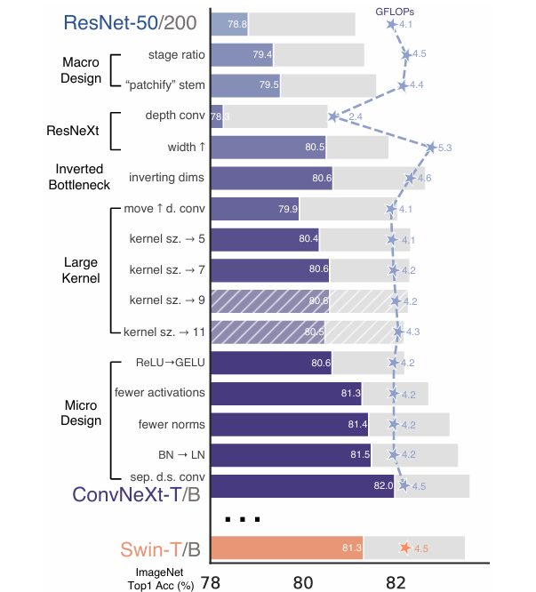 Figure 1. The hyperparameter tuning results done on the original ResNet architecture [1].
There were two ResNet variants used in their experiments: ResNet-50 and ResNet-200 (shown in purple and gray, respectively). Let’s now focus on the results obtained from tuning the ResNet-50 architecture. Based on the figure, we can see that this model initially obtained 78.8% accuracy on ImageNet dataset. They tuned this model until eventually it reached 82.0%, surpassing the state-of-the-art Swin-T architecture which only achieved 81.3% (the orange bar). This tuned version of the ResNet model is the one so-called ConvNeXt proposed in the paper. Their experiments on ResNet-200 confirm that the previous results are valid since its tuned version, i.e., ConvNeXt-B, also successfully surpasses the performance of Swin-B (the larger variant of Swin-T).
Macro Design
The first change made on the original ResNet was the macro design. If we take a closer look at Figure 2 below, we can see that a ResNet model essentially consists of four main stages, namely conv2_x , conv3_x , conv4_x and conv5_x , which each of them also comprises multiple bottleneck blocks. Talking more specifically about ResNet-50, the bottleneck blocks in each stage is repeated 3, 4, 6 and 3 times, respectively. Later on, I’ll refer to these numbers as stage ratio.
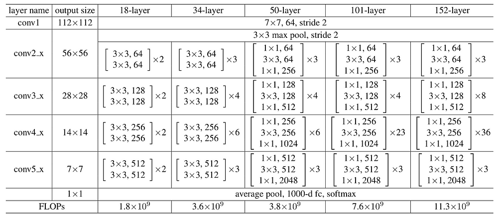 Figure 2. The ResNet architecture variants [3].
The authors of the ConvNeXt paper tried to change this stage ratio according to the Swin-T architecture, i.e., 1:1:3:1. Well, it’s actually 2:2:6:2 if you see the architectural details from the original Swin Transformer paper in Figure 3, but it’s basically just a derivation from the same ratio. By applying this configuration, authors obtained 0.6% improvement (from 78.8% to 79.4%). Thus, they decided to use 1:1:3:1 stage ratio for the upcoming experiments.
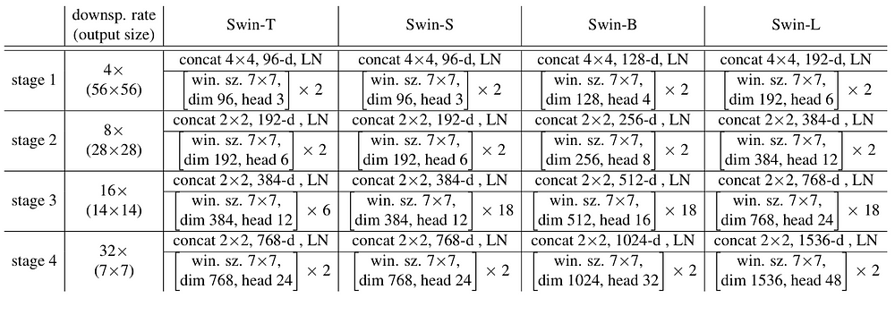 Figure 3. The Swin Transformer architecture variants [4].
Still related to macro design, changes were also made to the first convolution layer of ResNet. If you go back to Figure 2 (the conv1 row), you’ll see that it originally uses 7×7 kernel with stride 2, which reduces the image size from 224×224 to 112×112. Being inspired by Swin Transformer, authors also wanted to treat the input image as non-overlapping patches. Thus, they changed the kernel size to 4×4 and the stride to 4. This idea was actually adopted from the original ViT, where it uses 16×16 kernel with stride 16. One thing you need to know in ConvNeXt is that the resulting patches are treated as a standard image rather than a sequence. With this modification, the accuracy slightly improved from 79.4% to 79.5%. Hence, authors used this configuration for the first convolution layer in the next experiments.
ResNeXt-ification
As the macro design is done, the next thing authors did was to adopt the ResNeXt architecture, which was first proposed in a paper titled “ Aggregated Residual Transformations for Deep Neural Networks ” [5]. The idea of ResNeXt is that it basically applies group convolution to the bottleneck blocks of the ResNet architecture. In case you’re not yet familiar with group convolution, it essentially works by separating input channels into groups and performing convolution operations within each group independently, allowing faster computation as the number of groups increases. ConvNeXt adopts this idea by setting the number of groups to be the same as the number of kernels. This approach, which is commonly known as depthwise convolution , enables the network to obtain the lowest possible computational complexity. However, it is important to note that increasing the number of convolution groups like this leads to a reduction in accuracy as it lowers the model capacity to learn. Thus, the drop in accuracy to 78.3% was expected.
That wasn’t the end of the ResNeXt-ification section, though. In fact, the ResNeXt paper gives us a guidance that if we increase the number of groups, we also need to expand the width of the network, i.e., add more channels. Thus, ConvNeXt authors readjusted the number of kernels based on the one used in Swin-T. You can see in Figure 2 and 3 that ResNet originally uses 64, 128, 256 and 512 kernels in each stage, whereas Swin-T uses 96, 192, 384, and 768. Such an increase in the model width allows the network to significantly push the accuracy to 80.5%.
Inverted Bottleneck
Still with Figure 2, it is also seen that ResNet-50, ResNet-101, and ResNet-152 share the exact same bottleneck structure. For instance, the block at stage conv5_x consists of 3 convolution layers with 512, 512, and 2048 kernels, where the input of the first convolution is either 1024 (coming from the conv4_x stage) or 2048 (from the previous block in the conv5_x stage itself). These ResNet variations essentially follow the wide → narrow → wide structure, which is the reason that this block is called bottleneck. Instead of using a structure like this, ConvNeXt employs the inverted version of bottleneck, where it follows the narrow → wide → narrow structure adopted from the feed-forward layer of the Transformer architecture. In Figure 4 below (a) is the bottleneck block used in ResNet and (b) is the so-called inverted bottleneck block. By using this structure, the model accuracy increased from 80.5% to 80.6%.
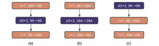 Figure 4. The bottleneck block in ResNeXt (a), the inverted bottleneck block (b), and the ConvNeXt block (c) [1].
Kernel Size
The next exploration was done on the kernel size inside the inverted bottleneck block. Before experimenting with different kernel sizes, further modification was done to the structure of the block, where authors swapped the order of the first and second layer such that the depthwise convolution is now placed at the beginning of the block as seen in Figure 4 (c). Thanks to this modification, the block is now called ConvNeXt block as it no longer completely resembles the original inverted bottleneck structure. This idea was actually adopted from Transformer, where the MSA (Multihead Self-Attention) layer is placed before the MLP layers. In the case of ConvNeXt, the depthwise convolution acts as the replacement of MSA, while the linear layers in MLP Transformers are replaced by pointwise convolutions. Simply moving up the depthwise convolution like this reduced the accuracy from 80.6% to 79.9%. However, this is acceptable because the current experiment set is still ongoing.
Experiments on the kernel size was then applied only on the depthwise convolution layer, leaving the remaining pointwise convolutions unchanged. Here authors tried to use different kernel sizes, where they found that 7×7 worked best as it successfully recovered the accuracy back to 80.6% with lower computational complexity (4.6 vs 4.2 GFLOPS). Interestingly, this kernel size matches the window dimensions in the Swin Transformer architecture, which corresponds to the patch size used in the self-attention mechanism. You can actually see this in Figure 3 where the window sizes in Swin Transformer variants are all 7×7.
Micro Design
The final aspect tuned in the paper is the so-called micro design , which essentially refers to the things related to the intricate details of the network. Similar to the previous ones, the parameters used here are mainly also adopted from Transformers. Authors initially replaced ReLU with GELU. Even though with this replacement the accuracy remained the same (80.6%), but they decided to go with this activation function for the subsequent experiments. The accuracy finally increased after the number of activation functions was reduced. Instead of applying GELU after each convolution layer in the ConvNeXt block, this activation function was placed only between the two pointwise convolutions. This modification allowed the network to boost the accuracy up to 81.3%, at which point this score was already on par with the Swin-T architecture while still having lower GFLOPS (4.2 vs 4.5).
Next, it is a common practice to use Conv-BN-ReLU structure in CNN-based architecture, which is exactly what ResNet implements as well. Instead of following this convention, authors decided to implement only a single batch normalization layer, which is placed before the first pointwise convolution layer. This change improved the accuracy to 81.4%, surpassing the accuracy of Swin-T by a little bit. Despite this achievement, parameter tuning was still continued by replacing batch norm with layer norm, which again raised the accuracy by 0.1% to 81.5%. All the modifications related to micro design resulted in the architecture shown in Figure 5 (the rightmost image). Here you can see how a ConvNeXt block differs from Swin Transformer and ResNet blocks.
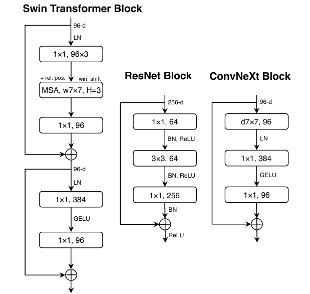 Figure 5. What the Swin-T, ResNet-50 and ConvNeXt-T blocks look like at the initial stage [1].
The last thing the authors did related to the micro design was applying separate downsampling layers. In the original ResNet architecture, the spatial dimension of a tensor reduces by half when we move from one stage to another. You can see in Figure 2 that initially ResNet accepts input of size 224×224 which then shrinks to 112×112, 56×56, 28×28, 14×14, and 7×7 at stage conv1 , conv2_x , conv3_x , conv4_x and conv5_x , respectively. Especially in conv2_x and the subsequent ones, the spatial dimension reduction is done by changing the stride parameter of the pointwise convolution to 2. Instead of doing so, ConvNeXt performs downsampling by placing another convolution layer right before the element-wise summation operation within the block. The kernel size and stride of this layer are set to 2, simulating a non-overlapping sliding window. In fact, it is mentioned in the paper that using this separate downsampling layer caused the accuracy to degrade instead. Nevertheless, authors managed to solve this issue by applying additional layer normalization layers at several parts of the network, i.e., before each downsampling layer, after the stem stage and after the global average pooling layer (right before the final output layer). With this tuning, authors successfully boosted the accuracy to 82.0%, which is much higher than Swin-T (81.3%) while still having the exact same GFLOPS (4.5).
And that’s basically all the modifications made on the original ResNet to create the ConvNeXt architecture. Don’t worry if it still feels a bit unclear for now — I believe things will become clearer as we get into the code.
···
ConvNeXt Implementation
Figure 6 below displays the details of the entire ConvNeXt-T architecture which we will later implement every single of its components one by one. Here you can also see how it differs from ResNet-50 and Swin-T, the two models that are comparable to ConvNeXt-T.
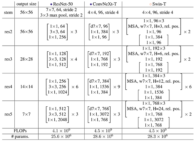 Figure 6. The details of the ResNet-50, ConvNeXt-T, and Swin-T architectures [1].
When it comes to the implementation, the first thing we need to do is to import the required modules. The only two we import here are the base
torch module and its nn submodule for loading neural network layers.
python
# Codeblock 1
import torch
import torch.nn as nn
ConvNeXt Block
Now let’s start with the ConvNeXt block. You can see in Figure 6 that the block structures in res2 , res3 , res4 , and res5 stages are basically the same, in which all of those correspond to the rightmost illustration in Figure 5. Thanks to these identical structures, we can implement them in a single class and use it repeatedly. Look at the Codeblock 2a and 2b below to see how I do that.
python
# Codeblock 2a
class ConvNeXtBlock(nn.Module):
    def __init__(self, num_channels):         #(1)
        super().__init__()
        hidden_channels = num_channels * 4    #(2)


        self.conv0 = nn.Conv2d(in_channels=num_channels,         #(3)
                               out_channels=num_channels,        #(4)
                               kernel_size=7,    #(5)
                               stride=1,
                               padding=3,        #(6)
                               groups=num_channels)              #(7)

        self.norm = nn.LayerNorm(normalized_shape=num_channels)  #(8)

        self.conv1 = nn.Conv2d(in_channels=num_channels,         #(9)
                               out_channels=hidden_channels,
                               kernel_size=1,
                               stride=1,
                               padding=0)

        self.gelu = nn.GELU()  #(10)

        self.conv2 = nn.Conv2d(in_channels=hidden_channels,      #(11)
                               out_channels=num_channels,
                               kernel_size=1,
                               stride=1,
                               padding=0)
I decided to name this class ConvNeXtBlock. You can see at line #(1) in the above codeblock that this class accepts num_channels as the only parameter, in which it denotes both the number of input and output channels. Remember that a ConvNeXt block follows the pattern of the inverted bottleneck structure, i.e., narrow → wide → narrow. If you take a closer look at Figure 6, you’ll notice that the wide part is 4 times larger than the narrow part. Thus, we set the value of the hidden_channels variable accordingly (#(2)).
Next, we initialize 3 convolution layers which I refer to them as conv0, conv1 and conv2. Every single of these convolution layers has their own specifications. For conv0, we set the number of input and output channels to be the same, which is the reason that both its in_channels and out_channels parameters are set to num_channels (#(3–4)). We set the kernel size of this layer to 7×7 (#(5)). Given this specification, we need to set the padding size to 3 in order to retain the spatial dimension (#(6)). Don’t forget to set the groups parameter to num_channels because we want this to be a depthwise convolution layer (#(7)). On the other hand, the conv1 layer (#(9)) is responsible to increase the number of image channels, whereas the subsequent conv2 layer (#(11)) is employed to shrink the tensor back to the original channel count. It is important to note that conv1 and conv2 are both using 1×1 kernel size, which essentially means that it only works by combining information along the channel dimension. Additionally, here we also need to initialize layer norm (#(8)) and GELU activation function (#(10)) as the replacement for batch norm and ReLU.
As all layers required in the ConvNeXtBlock have been initialized, what we need to do next is to define the flow of the tensor in the forward() method below.
python
# Codeblock 2b
    def forward(self, x):
        residual = x                 #(1)
        print(f'x & residual\t: {x.size()}')

        x = self.conv0(x)
        print(f'after conv0\t: {x.size()}')

        x = x.permute(0, 2, 3, 1)    #(2)
        print(f'after permute\t: {x.size()}')

        x = self.norm(x)
        print(f'after norm\t: {x.size()}')

        x = x.permute(0, 3, 1, 2)    #(3)
        print(f'after permute\t: {x.size()}')

        x = self.conv1(x)
        print(f'after conv1\t: {x.size()}')

        x = self.gelu(x)
        print(f'after gelu\t: {x.size()}')

        x = self.conv2(x)
        print(f'after conv2\t: {x.size()}')

        x = x + residual             #(4)
        print(f'after summation\t: {x.size()}')

        return x
What we basically do in the above code is just passing the tensor to each layer we defined earlier sequentially. However, there are two things I need to highlight here. First, we need to store the original input tensor to the residual variable (#(1)), in which it will skip over all operations within the ConvNeXt block. Secondly, remember that layer norm is commonly used for sequential data, where it typically has a different shape from that of image data. Due to this reason, we need to adjust the tensor dimension such that the shape becomes (N, H, W, C) (#(2)) before we actually perform the layer normalization operation. Afterwards, don’t forget to permute this tensor back to (N, C, H, W) (#(3)). The resulting tensor is then passed through the remaining layers before being summed with the residual connection (#(4)).
To check if our ConvNeXtBlock class works properly, we can test it using the Codeblock 3 below. Here we are going to simulate the block used in res2 stage. So, we set the num_channels parameter to 96 (#(1)) and create a dummy tensor which we assume as a batch of single image of size 56×56 (#(2)).
python
# Codeblock 3
convnext_block_test = ConvNeXtBlock(num_channels=96)  #(1)
x_test = torch.rand(1, 96, 56, 56)  #(2)

out_test = convnext_block_test(x_test)
Below is what the resulting output looks like. Talking about the internal flow, it seems like all layers we stacked earlier work properly. At line #(1) in the output below we can see that the tensor dimension changed to 1×56×56×96 (N, H, W, C) after being permuted. This tensor size then changed back to 1×96×56×56 (N, C, H, W) after the second permute operation (#(2)). Next, the conv1 layer successfully expanded the number of channels to be 4 times greater than the input (#(3)) which was then reduced back to the original channel count (#(4)). Here you can see that the tensor shape at the first and the last layer are exactly the same, allowing us to stack multiple ConvNeXt blocks as many as we want.
python
# Codeblock 3 Output
x & residual    : torch.Size([1, 96, 56, 56])
after conv0     : torch.Size([1, 96, 56, 56])
after permute   : torch.Size([1, 56, 56, 96])    #(1)
after norm      : torch.Size([1, 56, 56, 96])
after permute   : torch.Size([1, 96, 56, 56])    #(2)
after conv1     : torch.Size([1, 384, 56, 56])   #(3)
after gelu      : torch.Size([1, 384, 56, 56])
after conv2     : torch.Size([1, 96, 56, 56])    #(4)
after summation : torch.Size([1, 96, 56, 56])
···
ConvNeXt Block Transition
The next component I want to implement is the one I refer to as the ConvNeXt block transition. The idea of this block is actually similar to the ConvNeXt block we implemented earlier, except that this transition block is used when we are about to move from a stage to the subsequent one. More specifically, this block will later be employed as the first ConvNeXt block in each stage (except res2). The reason I implement it in separate class is that there are some intricate details that differ from the ConvNeXt block. Additionally, it is worth noting that the term transition is not officially used in the paper. Rather, it’s just the word I use on my own to describe this idea. — I actually also used this technique back when I write about the smaller ResNet version, i.e., ResNet-18 and ResNet-34. Click on the link at reference number [6] at the end of this article if you’re interested to read that one.
python
# Codeblock 4a
class ConvNeXtBlockTransition(nn.Module):
    def __init__(self, in_channels, out_channels):  #(1)
        super().__init__()
        hidden_channels = out_channels * 4

        self.projection = nn.Conv2d(in_channels=in_channels,      #(2)
                                    out_channels=out_channels,
                                    kernel_size=1,
                                    stride=2,
                                    padding=0)

        self.conv0 = nn.Conv2d(in_channels=in_channels,
                               out_channels=out_channels,
                               kernel_size=7,
                               stride=1,
                               padding=3,
                               groups=in_channels)

        self.norm0 = nn.LayerNorm(normalized_shape=out_channels)

        self.conv1 = nn.Conv2d(in_channels=out_channels,
                               out_channels=hidden_channels,
                               kernel_size=1,
                               stride=1,
                               padding=0)

        self.gelu = nn.GELU()

        self.conv2 = nn.Conv2d(in_channels=hidden_channels,
                               out_channels=out_channels,
                               kernel_size=1,
                               stride=1,
                               padding=0)

        self.norm1 = nn.LayerNorm(normalized_shape=out_channels)  #(3)

        self.downsample = nn.Conv2d(in_channels=out_channels,     #(4)
                                    out_channels=out_channels,
                                    kernel_size=2,
                                    stride=2)
The first difference you might notice here is the input of the __init__() method, which in this case we separate the number of input and output channels into two parameters as seen at line #(1) in Codeblock 4a. This is essentially done because we need this block to take the output tensor from the previous stage which has different number of channels from that of the one to be generated in the subsequent stage. Referring to Figure 6, for example, if we were to create the first ConvNeXt block in res3 stage, we need to configure it such that it accepts a tensor of 96 channels from res2 and returns another tensor with 192 channels.
Secondly, here we implement the separate downsample layer I explained earlier (#(4)) alongside the corresponding layer norm to be placed before it (#(3)). As the name suggests, this layer is employed to reduce the spatial dimension of the image by half.
Third, we initialize the so-called projection layer at line #(2). In the ConvNeXtBlock we created earlier, this layer is not necessary because the input and output tensor is exactly the same. In the case of transition block, the image spatial dimension is reduced by half, while at the same time the number of output channels is doubled. This projection layer is responsible to adjust the dimension of the residual connection in order to match it with the one from the main flow, allowing element-wise operation to be performed.
The forward() method in the Codeblock 4b below is also similar to the one belongs to the ConvNeXtBlock class, except that here the residual connection needs to be processed with the projection layer (#(1)) while the main tensor requires to be downsampled (#(2)) before the summation is done at line #(3).
python
# Codeblock 4b
    def forward(self, x):
        print(f'original\t\t: {x.size()}')

        residual = self.projection(x)  #(1)
        print(f'residual after proj\t: {residual.size()}')

        x = self.conv0(x)
        print(f'after conv0\t\t: {x.size()}')

        x = x.permute(0, 2, 3, 1)
        print(f'after permute\t\t: {x.size()}')

        x = self.norm0(x)
        print(f'after norm1\t\t: {x.size()}')

        x = x.permute(0, 3, 1, 2)
        print(f'after permute\t\t: {x.size()}')

        x = self.conv1(x)
        print(f'after conv1\t\t: {x.size()}')

        x = self.gelu(x)
        print(f'after gelu\t\t: {x.size()}')

        x = self.conv2(x)
        print(f'after conv2\t\t: {x.size()}')

        x = x.permute(0, 2, 3, 1)
        print(f'after permute\t\t: {x.size()}')

        x = self.norm1(x)
        print(f'after norm1\t\t: {x.size()}')

        x = x.permute(0, 3, 1, 2)
        print(f'after permute\t\t: {x.size()}')

        x = self.downsample(x)  #(2)
        print(f'after downsample\t: {x.size()}')

        x = x + residual  #(3)
        print(f'after summation\t\t: {x.size()}')

        return x
Now let’s test the ConvNeXtBlockTransition class above using the following codeblock. Suppose we are about to implement the first ConvNeXt block in stage res3. To do so, we can simply instantiate the transition block with in_channels=96 and out_channels=192 before eventually passing a dummy tensor of size 1×96×56×56 through it.
python
# Codeblock 5
convnext_block_transition_test = ConvNeXtBlockTransition(in_channels=96,
                                                         out_channels=192)
x_test = torch.rand(1, 96, 56, 56)

out_test = convnext_block_transition_test(x_test)
markup
# Codeblock 5 Outputoriginal : torch.Size([1, 96, 56, 56])residual after proj : torch.Size([1, 192, 28, 28]) #(1)after conv0 : torch.Size([1, 192, 56, 56]) #(2)after permute : torch.Size([1, 56, 56, 192])after norm0 : torch.Size([1, 56, 56, 192])after permute : torch.Size([1, 192, 56, 56])after conv1 : torch.Size([1, 768, 56, 56])after gelu : torch.Size([1, 768, 56, 56])after conv2 : torch.Size([1, 192, 56, 56]) #(3)after permute : torch.Size([1, 56, 56, 192])after norm1 : torch.Size([1, 56, 56, 192])after permute : torch.Size([1, 192, 56, 56])after downsample : torch.Size([1, 192, 28, 28]) #(4)after summation : torch.Size([1, 192, 28, 28]) #(5)
You can see in the resulting output that our projection layer directly maps the 1×96×56×56 residual tensor to 1×192×28×28 as shown at line #(1). Meanwhile, the main tensor x needs to be processed by the other layers we initialized earlier to achieve this shape. The steps we performed from line #(2) to #(3) on the x tensor are basically the same as those in the ConvNeXtBlock class. At this point we already got the number of channels matches our need (192). The spatial dimension is then reduced after the tensor being processed by the downsample layer (#(4)). As the tensor dimensions of x and residual have matched, we can finally perform the element-wise summation (#(5)).
···
The Entire ConvNeXt Architecture
As we got ConvNeXtBlock and ConvNeXtBlockTransition classes ready to use, we can now start to construct the entire ConvNeXt architecture. Before we do that, I would like to introduce some config parameters first. See the Codeblock 6 below.
python
# Codeblock 6
IN_CHANNELS  = 3     #(1)
IMAGE_SIZE   = 224   #(2)

NUM_BLOCKS   = [3, 3, 9, 3]         #(3)
OUT_CHANNELS = [96, 192, 384, 768]  #(4)
NUM_CLASSES  = 1000  #(5)
The first one is the dimension of the input image. As shown at line #(1) and #(2), here we set in_channels to 3 and image_size to 224 since by default ConvNeXt accepts a batch of RGB images of that size. The next ones are related to the model configuration. In this case, I set the number of ConvNeXt blocks of each stage to [3, 3, 9, 3] (#(3)) and the corresponding number of output channels to [96, 192, 384, 768] (#(4)) since I want to implement the ConvNeXt-T variant. You can actually change these numbers according to the configuration provided by the original paper shown in Figure 7. Finally, we set the number of neurons of the output channel to 1000, which corresponds to the number of classes in the dataset we train the model on (#(5)).
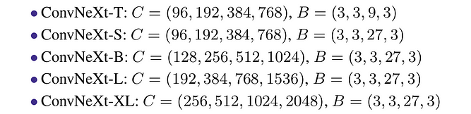 Figure 7. The ConvNeXt variants [1].
We will now implement the entire architecture in the
ConvNeXt class shown in Codeblock 7a and 7b below. The following __init__() method might seem a bit complicated at glance, but don’t worry as I’ll explain it thoroughly.
python
# Codeblock 7a
class ConvNeXt(nn.Module):
    def __init__(self):
        super().__init__()

        self.stem = nn.Conv2d(in_channels=IN_CHANNELS,    #(1)
                              out_channels=OUT_CHANNELS[0],
                              kernel_size=4,
                              stride=4,
                             )

        self.normstem = nn.LayerNorm(normalized_shape=OUT_CHANNELS[0])  #(2)

        #(3)
        self.res2 = nn.ModuleList()
        for _ in range(NUM_BLOCKS[0]):
            self.res2.append(ConvNeXtBlock(num_channels=OUT_CHANNELS[0]))

        #(4)
        self.res3 = nn.ModuleList([ConvNeXtBlockTransition(in_channels=OUT_CHANNELS[0],
                                                           out_channels=OUT_CHANNELS[1])])
        for _ in range(NUM_BLOCKS[1]-1):
            self.res3.append(ConvNeXtBlock(num_channels=OUT_CHANNELS[1]))

        #(5)
        self.res4 = nn.ModuleList([ConvNeXtBlockTransition(in_channels=OUT_CHANNELS[1],
                                                           out_channels=OUT_CHANNELS[2])])
        for _ in range(NUM_BLOCKS[2]-1):
            self.res4.append(ConvNeXtBlock(num_channels=OUT_CHANNELS[2]))

        #(6)
        self.res5 = nn.ModuleList([ConvNeXtBlockTransition(in_channels=OUT_CHANNELS[2],
                                                           out_channels=OUT_CHANNELS[3])])
        for _ in range(NUM_BLOCKS[3]-1):
            self.res5.append(ConvNeXtBlock(num_channels=OUT_CHANNELS[3]))


        self.avgpool = nn.AdaptiveAvgPool2d(output_size=(1,1))  #(7)
        self.normpool = nn.LayerNorm(normalized_shape=OUT_CHANNELS[3])  #(8)
        self.fc = nn.Linear(in_features=OUT_CHANNELS[3],        #(9)
                            out_features=NUM_CLASSES)

        self.relu = nn.ReLU()
The first thing we do here is initializing the stem stage (#(1)), which is essentially just a convolution layer with 4×4 kernel size and stride 4. This configuration will effectively reduce the image size to be 4 times smaller, where every single pixel in the output tensor represents a 4×4 patch in the input tensor. For the subsequent stages, we need to wrap the corresponding ConvNeXt blocks with nn.ModuleList(). For stage res3 (#(4)), res4 (#(5)) and res5 (#(6)) we place ConvNeXtBlockTransition at the beginning of each list as a “bridge” between stages. We don’t do this for stage res2 since the tensor produced by the stem stage is already compatible with it (#(3)). Next, we initialize an nn.AdaptiveAvgPool2d layer, which will be used to reduce the spatial dimensions of the tensor to 1x1 by computing the mean across each channel (#(7)). In fact, this is the exact same process used by ResNet to prepare the tensor from the last convolution layer so that it matches the shape required by the subsequent output layer (#(9)). Additionally, don’t forget to initialize two layer normalization layers which I refer to as normstem (#(2)) and normpool (#(8)), in which these two layers will then be placed right after the stem stage and the avgpool layer.
The forward() method is pretty straightforward. All we need to do in the following code is just to place the layers one after another. Keep in mind that since the ConvNeXt blocks are stored in lists, we need to call them iteratively with loops as seen at line #(1–4). Additionally, don’t forget to reshape the tensor produced by the nn.AdaptiveAvgPool2d layer (#(5)) so that it will be compatible with the subsequent fully-connected layer (#(6)).
python
# Codeblock 7b
    def forward(self, x):
        print(f'original\t: {x.size()}')

        x = self.relu(self.stem(x))
        print(f'after stem\t: {x.size()}')

        x = x.permute(0, 2, 3, 1)
        print(f'after permute\t: {x.size()}')

        x = self.normstem(x)
        print(f'after normstem\t: {x.size()}')

        x = x.permute(0, 3, 1, 2)
        print(f'after permute\t: {x.size()}')

        print()
        for i, block in enumerate(self.res2):    #(1)
            x = block(x)
            print(f'after res2 #{i}\t: {x.size()}')

        print()
        for i, block in enumerate(self.res3):    #(2)
            x = block(x)
            print(f'after res3 #{i}\t: {x.size()}')

        print()
        for i, block in enumerate(self.res4):    #(3)
            x = block(x)
            print(f'after res4 #{i}\t: {x.size()}')

        print()
        for i, block in enumerate(self.res5):    #(4)
            x = block(x)
            print(f'after res5 #{i}\t: {x.size()}')

        print()
        x = self.avgpool(x)
        print(f'after avgpool\t: {x.size()}')

        x = x.permute(0, 2, 3, 1)
        print(f'after permute\t: {x.size()}')

        x = self.normpool(x)
        print(f'after normpool\t: {x.size()}')

        x = x.permute(0, 3, 1, 2)
        print(f'after permute\t: {x.size()}')

        x = x.reshape(x.shape[0], -1)             #(5)
        print(f'after reshape\t: {x.size()}')

        x = self.fc(x)
        print(f'after fc\t: {x.size()}')          #(6)

        return x
Now for the moment of truth, let’s see if we have correctly implemented the entire ConvNeXt model by running the following code. Here I try to pass a tensor of size 1×3×224×224 to the network, simulating a batch of a single RGB image of size 224×224.
python
# Codeblock 8
convnext_test = ConvNeXt()

x_test   = torch.rand(1, IN_CHANNELS, IMAGE_SIZE, IMAGE_SIZE)
out_test = convnext_test(x_test)
You can see in the following output that it looks like our implementation is correct as the behavior of the network aligns with the architectural design shown in Figure 6. The spatial dimension of the image gradually gets smaller as we get deeper into the network, and at the same time the number of channels increases instead thanks to the ConvNeXtBlockTransition blocks we placed at the beginning of stage res3 (#(1)), res4 (#(2)), and res5 (#(3)). The avgpool layer then correctly downsampled the spatial dimension to 1×1 (#(4)), allowing it to be connected to the output layer (#(5)).
markup
# Codeblock 8 Outputoriginal : torch.Size([1, 3, 224, 224])after stem : torch.Size([1, 96, 56, 56])after permute : torch.Size([1, 56, 56, 96])after normstem : torch.Size([1, 56, 56, 96])after permute : torch.Size([1, 96, 56, 56])after res2 #0 : torch.Size([1, 96, 56, 56])after res2 #1 : torch.Size([1, 96, 56, 56])after res2 #2 : torch.Size([1, 96, 56, 56])after res3 #0 : torch.Size([1, 192, 28, 28]) #(1)after res3 #1 : torch.Size([1, 192, 28, 28])after res3 #2 : torch.Size([1, 192, 28, 28])after res4 #0 : torch.Size([1, 384, 14, 14]) #(2)after res4 #1 : torch.Size([1, 384, 14, 14])after res4 #2 : torch.Size([1, 384, 14, 14])after res4 #3 : torch.Size([1, 384, 14, 14])after res4 #4 : torch.Size([1, 384, 14, 14])after res4 #5 : torch.Size([1, 384, 14, 14])after res4 #6 : torch.Size([1, 384, 14, 14])after res4 #7 : torch.Size([1, 384, 14, 14])after res4 #8 : torch.Size([1, 384, 14, 14])after res5 #0 : torch.Size([1, 768, 7, 7]) #(3)after res5 #1 : torch.Size([1, 768, 7, 7])after res5 #2 : torch.Size([1, 768, 7, 7])after avgpool : torch.Size([1, 768, 1, 1]) #(4)after permute : torch.Size([1, 1, 1, 768])after normpool : torch.Size([1, 1, 1, 768])after permute : torch.Size([1, 768, 1, 1])after reshape : torch.Size([1, 768])after fc : torch.Size([1, 1000]) #(5)
···
Ending
Well, that was pretty much everything about the theory and the implementation of the ConvNeXt architecture. Again, I do acknowledge that the code I demonstrate above might not fully capture everything since this article is intended to cover the general idea of the model. So, I highly recommend you read the original implementation by Meta’s researchers [2] if you want to know more about the intricate details.
I hope you find this article useful. Thanks for reading!
P.S. the notebook used in this article is available on my GitHub repo. See the link at reference number [7].
···
References
[1] Zhuang Liu et al. A ConvNet for the 2020s. Arxiv. https://arxiv.org/pdf/2201.03545 [Accessed January 18, 2025].
[2] facebookresearch. ConvNeXt. GitHub. https://github.com/facebookresearch/ConvNeXt/blob/main/models/convnext.py [Accessed January 18, 2025].
[3] Kaiming He et al. Deep Residual Learning for Image Recognition. Arxiv. https://arxiv.org/pdf/1512.03385 [Accessed January 18, 2025].
[4] Ze Liu et al. Swin Transformer: Hierarchical Vision Transformer using Shifted Windows. Arxiv. https://arxiv.org/pdf/2103.14030 [Accessed January 18, 2025].
[5] Saining Xie et al. Aggregated Residual Transformations for Deep Neural Networks. Arxiv. https://arxiv.org/pdf/1611.05431 [Accessed January 18, 2025].
[6] Muhammad Ardi. Paper Walkthrough: Residual Network (ResNet). Python in Plain English. https://python.plainenglish.io/paper-walkthrough-residual-network-resnet-62af58d1c521 [Accessed January 19, 2025].
[7] MuhammadArdiPutra. The CNN That Challenges ViT — ConvNeXt. GitHub. https://github.com/MuhammadArdiPutra/medium_articles/blob/main/The CNN That Challenges ViT - ConvNeXt.ipynb [Accessed January 24, 2025].
Register Now to Continue Reading
Unlock Towards Data Science with a Free Account
All articles on Towards Data Science are available to registered users. Create a free account today to access this article and thousands more.
Register for freeSign in to your account
 Written By
Deep learning storyteller
See all from Muhammad Ardi Putra
Deep DivesArtificial IntelligenceComputer VisionImage ProcessingNeural Network
Share This Article
Towards Data Science is a community publication. Submit your insights to reach our global audience and earn through the TDS Author Payment Program.
Write for TDS
Related Articles
Artificial Intelligence
I'm looking back at my projects from my Data Science program at Flatiron and reviewing the ethical concerns that each has...
Mike Erb
November 3, 20209 min read
Artificial Intelligence
How sensor hubs on smartphones helped bring artificial intelligence to the edge
Kenneth Joel
September 28, 20224 min read
Robotics
3D simulations and movement control with PyBullet
Mauro Di Pietro
October 23, 20259 min read
Programming
How to make use of the Fourier Transformation to remove image elements
Tonichi Edeza
January 28, 20213 min read
Deep Learning
Half of the solution is comprehending your problem, but half of the comprehension is knowing how complicated it is
Houssem Ben Braiek
January 31, 20226 min read
Artificial Intelligence
A journey into the evolution of Big Data Compute Platforms like Hadoop and Spark. Sharing my perspective on where we were, where we are...
Manoj Kukreja
December 27, 20207 min read
Artificial Intelligence
Yellowbrick for creating machine learning plots with less code
Rukshan Pramoditha
November 5, 202215 min read
Artificial Intelligence
Shedding the light on real-life's non-human-centric data in which a hidden nested class imbalance problem exists, which is -up to the...
Ahmed Masri
April 21, 20216 min read
Artificial Intelligence
An introduction to linear programming and how to solve it using the graphical and simplex algorithms
Egor Howell
July 24, 20236 min read
Your home for data science and AI. The world's leading publication for data science, data analytics, data engineering, machine learning, and artificial intelligence professionals.
Subscribe to Our NewsletterWrite For TDS•About•Advertise•Privacy Policy•Terms of Use
© Insight Media Group, LLC 2026•The New Stack•roadmap.sh•Creator Network
Recommended Articles
Close