Building a GPT Model from Scratch (Part 5): Fine-Tuning GPT-2 for Text Classification
How I adapted a pretrained GPT-2 model to classify SMS messages as spam or not spam.

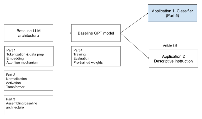
In the previous article, we loaded OpenAI’s pretrained GPT-2 weights into the model we had built from scratch. Now, we will adapt that model for text classification—specifically, identifying whether an SMS message is spam or not spam.
This requires three changes:
Data preparation: We need to standardize messages of different lengths using padding and truncation, and assign each message a binary label:
0for not spam and1for spam.Model architecture: We need to replace the original output layer, which produces
50,257vocabulary logits, with a smaller layer that produces two class logits.Training and evaluation: We need to calculate cross-entropy loss using the final sequence position and track classification accuracy separately.
Once these changes are in place, we will fine-tune the model on a public SMS spam dataset and test it on a few new messages.
Preparing the Data for Classification
The first part of the process remains familiar. We begin with a text message, tokenize it, and convert the tokens into token IDs that can be passed through the model.
Classification introduces two differences. First, messages can have very different lengths. Second, each message now has one label rather than a sequence of next-token targets.
Consider two messages that produce the following token IDs:
Message 1: [1212, 318, 257, 1332]
Message 2: [1026, 338, 257, 2392, 286, 2420, 290, 467]
The first message contains four token IDs, while the second contains eight. To combine them into a single training batch, they must have the same length. We therefore add padding to the shorter message:
Message 1: [1212, 318, 257, 1332, 50256, 50256, 50256, 50256]
Message 2: [1026, 338, 257, 2392, 286, 2420, 290, 467]
In this implementation, we reuse GPT-2’s end-of-text token, which has the token ID 50256, as the padding token. Shorter messages are padded, while messages longer than the selected maximum length are truncated.
The core logic inside the dataset class looks like this:
def __init__(self, csv_file, tokenizer, max_length=None, pad_token_id=50256):
    self.data = pd.read_csv(csv_file)
    self.encoded_texts = [tokenizer.encode(text) for text in self.data["Text"]]
    self.max_length = max_length or max(map(len, self.encoded_texts))

    self.encoded_texts = [tokens[:self.max_length] for tokens in self.encoded_texts]
    self.encoded_texts = [
        tokens + [pad_token_id] * (self.max_length - len(tokens))
        for tokens in self.encoded_texts
    ]
You can think of padding tokens as placeholders that fill the unused positions in shorter inputs. Technically, however, they are still token IDs that the model processes; they are not automatically ignored.
The second change is the training target. During next-token training, the target was another sequence of token IDs. For classification, every message receives one label:
0 → not spam
1 → spam
The model receives the tokenized message as input and learns to predict this single class.
Adapting the Output Layer for Classification
The second major change is in the model’s final output layer.
Our GPT-2 Small model produces a 768-dimensional representation at every token position. The original output layer converts each representation into 50,257 logits—one for every token in the GPT-2 vocabulary. These logits are used to predict which token should come next.
For classification, we no longer need an output for the entire vocabulary. We only need two class logits:
Next-token prediction:
768 dimensions → 50,257 vocabulary logits

Binary classification:
768 dimensions → 2 class logits
We first freeze the pretrained model parameters and then replace the original output layer with a new classification head:
for param in model.parameters():
    param.requires_grad = False

torch.manual_seed(123)
model.out_head = torch.nn.Linear(BASE_CONFIG["emb_dim"], 2)

for layer in (model.trf_blocks[-1], model.final_norm):
    for param in layer.parameters():
        param.requires_grad = True
The new output head is trainable by default. We also make the final transformer block and final normalization layer trainable.
The earlier layers retain the language patterns learned during pretraining, while the later layers can adapt those representations for spam classification. This is much more efficient than retraining the entire GPT-2 model from scratch.
Updating the Loss and Evaluation
The final change is in how we train and evaluate the model.
Ultimately, we care about classification accuracy: the percentage of messages correctly identified as spam or not spam. Accuracy itself, however, depends on selecting the class with the highest score. This is a discrete decision and does not provide the gradients needed to update the model.
We therefore train the model using cross-entropy loss and calculate accuracy separately. Cross-entropy compares the model’s class logits with the correct label and gives us a differentiable value that can be minimized during training.
There is also a difference in which outputs contribute to the loss:
Next-token prediction:
Loss is calculated across every token position

Text classification:
Loss is calculated using only the final sequence position
The model still produces two class logits at every position, but we select only the logits from the final position:
logits = model(input_batch)[:, -1, :]
loss = torch.nn.functional.cross_entropy(logits, target_batch)
Because GPT uses causal attention, the representation at the final position can use information from all the positions that came before it. It therefore contains information accumulated across the sequence.
For a padded input, this final position will usually contain a padding token. Its representation can still draw on the actual message tokens before it, although it may also be influenced by the padding positions.
It is worth clarifying that the final token does not literally contain the answer. The actual label—0 or 1—is stored separately. We simply compare that label with the two class logits produced at the final sequence position.
During evaluation, we select the class with the larger logit and check whether it matches the actual label.
Training on an SMS Spam Dataset
With these changes in place, we are ready to fine-tune the model.
I used the public SMS Spam Collection dataset, which contains messages labelled as either ham, meaning not spam, or spam.
df = pd.read_csv(
    data_file_path, sep="\t", header=None, names=["Label", "Text"]
)
A small preview of the data looks like this:
| Index | Label | Text |
|---|---|---|
| 0 | ham | Go until Jurong Point, crazy… Available only… |
| 1 | ham | Ok lar… Joking wif u oni… |
| 2 | spam | Free entry in 2 a wkly comp to win FA Cup fina… |
| … | … | … |
| 5570 | ham | The guy did some bitching, but I acted like I'd… |
| 5571 | ham | Rofl. It's true to its name. |
File used in this experiment: 5,572 messages
The current UCI dataset page lists 5,574 instances, while the downloaded file used in this notebook contains 5,572 rows. Dataset counts can therefore vary slightly depending on the distributed version of the file.
The data used here is heavily imbalanced:
Not spam: 4,825
Spam:       747
A classifier trained directly on this data could achieve high accuracy by predicting not spam most of the time. To create a more balanced experiment, I retained all 747 spam messages and randomly selected the same number of non-spam messages:
spam = df[df["Label"] == "spam"]
ham = df[df["Label"] == "ham"].sample(len(spam), random_state=123)

df = pd.concat([ham, spam]).sample(frac=1, random_state=123)
df["Label"] = df["Label"].map({"ham": 0, "spam": 1})
This gives us 1,494 examples, evenly divided between the two classes. I then split them into training, validation, and test sets using a 70% / 10% / 20% split.
The training set updates the model’s trainable weights. The validation set helps us monitor performance during training, while the test set gives us a final measure using data the model did not see during training.
Fine-Tuning the Model
I trained the model for five epochs using AdamW:
torch.manual_seed(123)
optimizer = torch.optim.AdamW(
    (p for p in model.parameters() if p.requires_grad),
    lr=1e-5, weight_decay=0.1
)

results = train_classifier_simple(
    model, train_loader, val_loader, optimizer, device,
    num_epochs=5, eval_freq=50, eval_iter=5
)
A shortened version of the training output is shown below:
Epoch 1, Step 0:   Train Loss 3.0852, Val Loss 2.4835
Epoch 1, Step 50:  Train Loss 0.5300, Val Loss 0.4591
...
Epoch 5, Step 550: Train Loss 0.0246, Val Loss 0.0727
Epoch 5, Step 600: Train Loss 0.1635, Val Loss 0.1263

Checkpoint train accuracy: 95.0%
Checkpoint val accuracy:   97.5%
Training time: 641.97 minutes
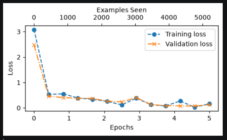
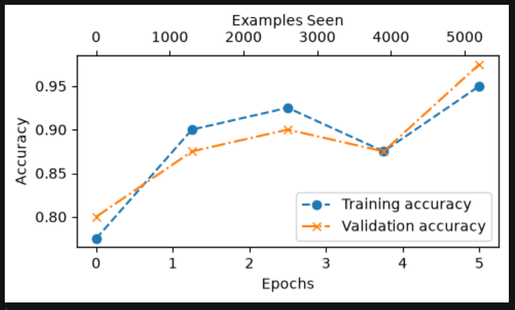
On my local setup, completing five epochs took approximately 642 minutes—or a little over ten hours. GPT-2 Small may be small compared with modern commercial models, but fine-tuning it locally can still be computationally expensive.
Trying the Classifier
Once training was complete, I tested the model using two custom messages:
texts = [
    "Congratulations! You've won a free ticket to Bahamas. Call now to claim your prize.",
    "Hey, are we still on for dinner tonight?"
]

for text in texts:
    print(classify_review(
        text, model, tokenizer, device,
        max_length=train_dataset.max_length
    ))
The predictions were:
spam
not spam
The model correctly classified both examples.
Finally, I saved the trained weights so that I could reuse the classifier without running the full training process again:
torch.save(model.state_dict(), "spam_classifier.pth")
One Interesting Observation
While experimenting with custom messages, I noticed that the classifier generally performed better on longer, clearly spam-like messages than on very short inputs.
One possible reason is the way the inputs are prepared. Every message is padded to the same maximum length, and the classifier uses the representation at the final sequence position. A short message therefore contains many more padding tokens than a longer message.
This does not mean padding is necessarily the only reason for an incorrect prediction. However, it shows how preprocessing decisions can affect real-world model behaviour. A model may achieve reasonable test accuracy while still behaving differently on inputs whose length or writing style differs from the training data.
This is also an important product lesson: a single overall accuracy number does not tell us how a model will behave across every type of real-world input.
Conclusion
In this article, we converted our pretrained GPT-2 model from a next-token predictor into a binary text classifier.
We standardized inputs using padding and truncation, replaced the vocabulary output layer with a two-class classification head, froze most of the pretrained model, and updated the loss calculation to use the class logits from the final sequence position. We then fine-tuned the model on an SMS spam dataset and used it to classify new messages as spam or not spam.
In the next article, we will explore another application of the same model: instruction fine-tuning. Instead of selecting between a fixed set of classes, the model will learn to generate a useful response to an instruction.
After that, we will move into the experimentation phase and start changing different parts of the model to understand how architecture and training choices affect its behaviour.
References
Sebastian Raschka — Build a Large Language Model (From Scratch) The primary reference for this project, covering tokenization, attention, GPT-style model construction, pretraining, classification fine-tuning, and instruction fine-tuning. Book on Manning · Official companion repository
Aman Jain — LLMs From Scratch Project The code accompanying this article series, including the baseline model, GPT-2 weight loading, classification fine-tuning, and instruction fine-tuning. View the project on GitHub
UCI Machine Learning Repository — SMS Spam Collection The public SMS dataset used for the classification experiment. View the dataset
OpenAI — GPT-2 OpenAI’s official GPT-2 code, model configurations, tokenizer files, and released checkpoints. GPT-2 repository · GPT-2 paper