保留正文与补采附件。源页面当前未重新核验;具体限制见交付清单。
 We value your privacy
We use cookies to enhance your browsing experience, serve personalised ads or content, and analyse our traffic. By clicking "Accept All", you consent to our use of cookies.
Customise Reject All Accept All
Customise Consent Preferences
 We use cookies to help you navigate efficiently and perform certain functions. You will find detailed information about all cookies under each consent category below.
The cookies that are categorised as "Necessary" are stored on your browser as they are essential for enabling the basic functionalities of the site. ... Show more
NecessaryAlways Active
Necessary cookies are required to enable the basic features of this site, such as providing secure log-in or adjusting your consent preferences. These cookies do not store any personally identifiable data.
-
Cookie
BCTempID
-
Duration
10 minutes
-
Description
No description available.
-
Cookie
__cf_bm
-
Duration
1 hour
-
Description
This cookie, set by Cloudflare, is used to support Cloudflare Bot Management.
-
Cookie
AWSALBCORS
-
Duration
7 days
-
Description
Amazon Web Services set this cookie for load balancing.
-
Cookie
_cfuvid
-
Duration
session
-
Description
Cloudflare sets this cookie to track users across sessions to optimize user experience by maintaining session consistency and providing personalized services
-
Cookie
li_gc
-
Duration
6 months
-
Description
Linkedin set this cookie for storing visitor's consent regarding using cookies for non-essential purposes.
-
Cookie
__hssrc
-
Duration
session
-
Description
This cookie is set by Hubspot whenever it changes the session cookie. The __hssrc cookie set to 1 indicates that the user has restarted the browser, and if the cookie does not exist, it is assumed to be a new session.
-
Cookie
__hssc
-
Duration
1 hour
-
Description
HubSpot sets this cookie to keep track of sessions and to determine if HubSpot should increment the session number and timestamps in the __hstc cookie.
-
Cookie
wpEmojiSettingsSupports
-
Duration
session
-
Description
WordPress sets this cookie when a user interacts with emojis on a WordPress site. It helps determine if the user's browser can display emojis properly.
-
Cookie
BCSessionID
-
Duration
1 year 1 month 4 days
-
Description
Blueconic sets this cookie as a unique identifier for the BlueConic profile.
-
Cookie
_octo
-
Duration
1 year
-
Description
No description available.
-
Cookie
logged_in
-
Duration
1 year
-
Description
No description available.
-
Cookie
__Secure-YEC
-
Duration
past
-
Description
YouTube sets this cookie to stores the user's video player preferences using embedded YouTube video
-
Cookie
__eoi
-
Duration
6 months
-
Description
Description is currently not available.
-
Cookie
AWSALBTGCORS
-
Duration
7 days
-
Description
No description available.
-
Cookie
login-status-p
-
Duration
past
-
Description
Description is currently not available.
-
Cookie
AWSALBTG
-
Duration
7 days
-
Description
No description available.
-
Cookie
csrf_token
-
Duration
session
-
Description
No description available.
-
Cookie
token_v2
-
Duration
1 day
-
Description
Description is currently not available.
-
Cookie
D
-
Duration
1 year
-
Description
Description is currently not available.
-
Cookie
PHPSESSID
-
Duration
session
-
Description
This cookie is native to PHP applications. The cookie stores and identifies a user's unique session ID to manage user sessions on the website. The cookie is a session cookie and will be deleted when all the browser windows are closed.
-
Cookie
VISITOR_PRIVACY_METADATA
-
Duration
6 months
-
Description
YouTube sets this cookie to store the user's cookie consent state for the current domain.
-
Cookie
cookietest
-
Duration
session
-
Description
The cookietest cookie is typically used to determine whether the user's browser accepts cookies, essential for website functionality and user experience.
-
Cookie
__Host-airtable-session
-
Duration
1 year
-
Description
This cookie is used to enable us to integrate the services of Airtable.
-
Cookie
__Host-airtable-session.sig
-
Duration
1 year
-
Description
This cookie is used to enable us to integrate the services of Airtable.
-
Cookie
m
-
Duration
1 year 1 month 4 days
-
Description
Stripe sets this cookie for fraud prevention purposes. It identifies the device used to access the website, allowing the website to be formatted accordingly.
-
Cookie
BIGipServer*
-
Duration
session
-
Description
Marketo sets this cookie to collect information about the user's online activity and build a profile about their interests to provide advertisements relevant to the user.
-
Cookie
__cfruid
-
Duration
session
-
Description
Cloudflare sets this cookie to identify trusted web traffic.
-
Cookie
_GRECAPTCHA
-
Duration
6 months
-
Description
Google Recaptcha service sets this cookie to identify bots to protect the website against malicious spam attacks.
-
Cookie
__Secure-YNID
-
Duration
6 months
-
Description
Google cookie used to protect user security and prevent fraud, especially during the login process.
-
Cookie
cookieyes-consent
-
Duration
1 year
-
Description
CookieYes sets this cookie to remember users' consent preferences so that their preferences are respected on subsequent visits to this site. It does not collect or store any personal information about the site visitors.
Functional
Functional cookies help perform certain functionalities like sharing the content of the website on social media platforms, collecting feedback, and other third-party features.
-
Cookie
lidc
-
Duration
1 day
-
Description
LinkedIn sets the lidc cookie to facilitate data center selection.
-
Cookie
brw
-
Duration
1 year
-
Description
No description available.
-
Cookie
brwConsent
-
Duration
5 minutes
-
Description
Description is currently not available.
-
Cookie
WMF-Uniq
-
Duration
1 year
-
Description
Description is currently not available.
-
Cookie
loom_anon_comment
-
Duration
1 year
-
Description
No description available.
-
Cookie
loom_referral_video
-
Duration
session
-
Description
Description is currently not available.
-
Cookie
VISITOR_INFO1_LIVE
-
Duration
6 months
-
Description
A cookie set by YouTube to measure bandwidth that determines whether the user gets the new or old player interface.
-
Cookie
yt-remote-connected-devices
-
Duration
Never Expires
-
Description
YouTube sets this cookie to store the user's video preferences using embedded YouTube videos.
-
Cookie
ytidb::LAST_RESULT_ENTRY_KEY
-
Duration
Never Expires
-
Description
The cookie ytidb::LAST_RESULT_ENTRY_KEY is used by YouTube to store the last search result entry that was clicked by the user. This information is used to improve the user experience by providing more relevant search results in the future.
-
Cookie
yt-remote-device-id
-
Duration
Never Expires
-
Description
YouTube sets this cookie to store the user's video preferences using embedded YouTube videos.
-
Cookie
yt-remote-session-name
-
Duration
session
-
Description
The yt-remote-session-name cookie is used by YouTube to store the user's video player preferences using embedded YouTube video.
-
Cookie
yt-remote-fast-check-period
-
Duration
session
-
Description
The yt-remote-fast-check-period cookie is used by YouTube to store the user's video player preferences for embedded YouTube videos.
-
Cookie
yt-remote-session-app
-
Duration
session
-
Description
The yt-remote-session-app cookie is used by YouTube to store user preferences and information about the interface of the embedded YouTube video player.
-
Cookie
yt-remote-cast-available
-
Duration
session
-
Description
The yt-remote-cast-available cookie is used to store the user's preferences regarding whether casting is available on their YouTube video player.
-
Cookie
yt-remote-cast-installed
-
Duration
session
-
Description
The yt-remote-cast-installed cookie is used to store the user's video player preferences using embedded YouTube video.
-
Cookie
cp_session
-
Duration
3 months
-
Description
Codepen sets this cookie for Help systems found in the website.
-
Cookie
loid
-
Duration
1 year 1 month 4 days
-
Description
This cookie is set by the Reddit. The cookie enables the sharing of content from the website onto the social media platform.
Analytics
Analytical cookies are used to understand how visitors interact with the website. These cookies help provide information on metrics such as the number of visitors, bounce rate, traffic source, etc.
-
Cookie
__hstc
-
Duration
6 months
-
Description
Hubspot set this main cookie for tracking visitors. It contains the domain, initial timestamp (first visit), last timestamp (last visit), current timestamp (this visit), and session number (increments for each subsequent session).
-
Cookie
hubspotutk
-
Duration
6 months
-
Description
HubSpot sets this cookie to keep track of the visitors to the website. This cookie is passed to HubSpot on form submission and used when deduplicating contacts.
-
Cookie
_ga
-
Duration
1 year 1 month 4 days
-
Description
Google Analytics sets this cookie to calculate visitor, session and campaign data and track site usage for the site's analytics report. The cookie stores information anonymously and assigns a randomly generated number to recognise unique visitors.
-
Cookie
ga*
-
Duration
1 year 1 month 4 days
-
Description
Google Analytics sets this cookie to store and count page views.
-
Cookie
__Host-psifi.analyticsTrace
-
Duration
6 hours
-
Description
Description is currently not available.
-
Cookie
__Host-psifi.analyticsTraceV2
-
Duration
6 hours
-
Description
Description is currently not available.
-
Cookie
_gh_sess
-
Duration
session
-
Description
GitHub sets this cookie for temporary application and framework state between pages like what step the user is on in a multiple step form.
-
Cookie
YSC
-
Duration
session
-
Description
YSC cookie is set by Youtube and is used to track the views of embedded videos on Youtube pages.
-
Cookie
ajs_anonymous_id
-
Duration
1 year
-
Description
This cookie is set by Segment to count the number of people who visit a certain site by tracking if they have visited before.
-
Cookie
vuid
-
Duration
1 year 1 month 4 days
-
Description
Vimeo installs this cookie to collect tracking information by setting a unique ID to embed videos on the website.
Performance
Performance cookies are used to understand and analyse the key performance indexes of the website which helps in delivering a better user experience for the visitors.
-
Cookie
AWSALB
-
Duration
7 days
-
Description
AWSALB is an application load balancer cookie set by Amazon Web Services to map the session to the target.
-
Cookie
acq
-
Duration
past
-
Description
Description is currently not available.
-
Cookie
acq.sig
-
Duration
past
-
Description
Description is currently not available.
-
Cookie
ptc
-
Duration
2 years
-
Description
No description available.
Advertisement
Advertisement cookies are used to provide visitors with customised advertisements based on the pages you visited previously and to analyse the effectiveness of the ad campaigns.
-
Cookie
muc_ads
-
Duration
1 year 1 month 4 days
-
Description
Twitter sets this cookie to collect user behaviour and interaction data to optimize the website.
-
Cookie
guest_id_marketing
-
Duration
1 year 1 month 4 days
-
Description
Twitter sets this cookie to identify and track the website visitor.
-
Cookie
guest_id_ads
-
Duration
1 year 1 month 4 days
-
Description
Twitter sets this cookie to identify and track the website visitor.
-
Cookie
personalization_id
-
Duration
1 year 1 month 4 days
-
Description
Twitter sets this cookie to integrate and share features for social media and also store information about how the user uses the website, for tracking and targeting.
-
Cookie
guest_id
-
Duration
1 year 1 month 4 days
-
Description
Twitter sets this cookie to identify and track the website visitor. It registers if a user is signed in to the Twitter platform and collects information about ad preferences.
-
Cookie
bcookie
-
Duration
1 year
-
Description
LinkedIn sets this cookie from LinkedIn share buttons and ad tags to recognize browser IDs.
-
Cookie
__Secure-ROLLOUT_TOKEN
-
Duration
6 months
-
Description
YouTube sets this cookie to manage feature rollout and experimentation. It helps Google control which new features or interface changes are shown to users as part of testing and staged rollouts, ensuring consistent experience for a given user during an experiment.
-
Cookie
yt.innertube::nextId
-
Duration
Never Expires
-
Description
YouTube sets this cookie to register a unique ID to store data on what videos from YouTube the user has seen.
-
Cookie
yt.innertube::requests
-
Duration
Never Expires
-
Description
YouTube sets this cookie to register a unique ID to store data on what videos from YouTube the user has seen.
-
Cookie
session_tracker
-
Duration
session
-
Description
This cookie is set by the Reddit. This cookie is used to identify trusted web traffic. It also helps in adverstising on the website.
-
Cookie
edgebucket
-
Duration
session
-
Description
Reddit sets this cookie to save the information about a log-on Reddit user, for the purpose of advertisement recommendations and updating the content.
-
Cookie
did
-
Duration
1 year
-
Description
Arbor sets this cookie to show targeted ads to site visitors.This cookie expires after 2 months or 1 year.
Uncategorised
Other uncategorised cookies are those that are being analysed and have not been classified into a category as yet.
No cookies to display.
Reject All Save My Preferences Accept All
Toggle SearchToggle Mobile Navigation
Publish AI, ML & data-science insights to a global community of data professionals.
Sign inSubmit an Article
LatestEditor's PicksNewsletterShipAI
Write For TDS
LinkedInXToggle Search
Deep Learning
Efficient Image Segmentation Using PyTorch: Part 2
A CNN-based model
Dhruv Matani
June 27, 202312 min read
This is the second part of the 4-part series to implement image segmentation step by step from scratch using deep learning techniques in PyTorch. This part will focus on implementing a baseline image segmentation Convolutional Neural Network (CNN) model.
Co-authored with Naresh Singh
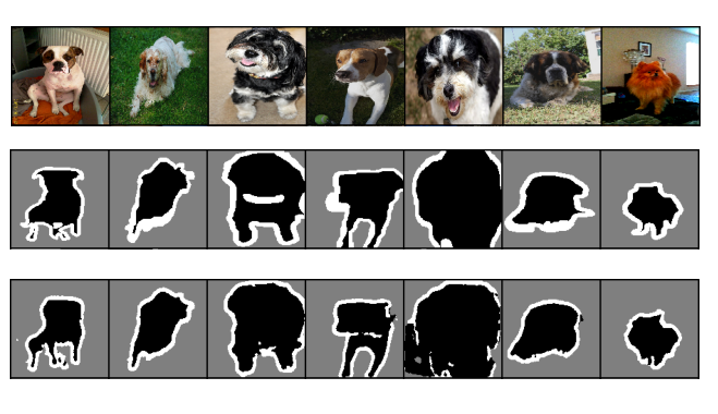 Figure 1: Result of running image segmentation using a CNN. In order from top to bottom, input images, ground truth segmentation masks, predicted segmentation masks. Source: Author(s)
Learn this step by step with the interactive Machine Learning roadmap.
Article outline
In this article, we will implement a Convolutional Neural Network (CNN) based architecture called SegNet which will assign each pixel in an input image to a corresponding pet such as a cat or a dog. The pixels which don't belong to any pet will be classified as background pixels. We will build and train this model on the Oxford Pets dataset using PyTorch to develop a sense of what it takes to deliver a successful image segmentation task. The model building process will be hands-on where we will discuss in detail the role of each layer in our model. The article will contain plenty of references to research papers and articles for further learning.
Throughout this article, we will reference the code and results from this notebook. If you wish to reproduce the results, you'll need a GPU to ensure that the notebook completes running in a reasonable amount of time.
Articles in this series
This series is for readers at all experience levels with deep learning. If you want to learn about the practice of deep learning and vision AI along with some solid theory and hands-on experience, you've come to the right place! This is expected to be a 4-part series with the following articles:
- Concepts and Ideas
- A CNN-based model (this article)
- Depthwise separable convolutions
- A Vision Transformer-based model
Let's start this discussion with a short introduction to the Convolution layers and a few other layers that are typically used together as a convolution block.
Conv-BatchNorm-ReLU and Max Pooling/Unpooling
A convolution, batch-normalization, ReLU block is the holy trinity of vision AI. You'll see it used frequently with CNN-based vision AI models. Each of these terms stands for a distinct layer implemented in PyTorch. The convolution layer is responsible for performing a cross-correlation operation of learned filters on the input tensor. Batch Normalization centers the elements in the batch to zero mean and unit variance, and ReLU is a non-linear activation function that keeps just the positive values in the input.
A typical CNN progressively reduces the input spatial dimensions as layers are stacked. The motivation behind the reduction of spatial dimensions is discussed in the next section. This reduction is achieved by pooling the neighboring values using a simple function such as max or average. We will discuss this further in the Max-Pooling section. In classification problems, the stack of Conv-BN-ReLU-Pool blocks is followed by a classification head which predicts the probability that input belongs to one of the target classes. Some sets of problems such as Semantic Segmentation require per-pixel prediction. For such cases, a stack of upsampling blocks are appended after the downsampling blocks to project their output to the required spatial dimension. The upsampling blocks are nothing but Conv-BN-ReLU-Unpool blocks which replace the pooling layer with an un-pooling layer. We will talk more about un-pooling in the Max-Pooling section.
Now, let's further elaborate on the motivation behind convolution layers.
Convolution
Convolutions are the basic building blocks of vision AI models. They are used heavily in computer vision and have historically been used to implement vision transformations such as:
- Edge detection
- Image blurring and sharpening
- Embossing
- Intensification
A convolution operation is an elementwise multiplication and aggregation of two matrices. An example convolution operation is shown in Figure 2.
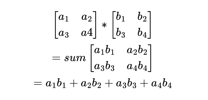 Figure 2: An illustration of the convolution operation. Source: Author(s)
In a deep learning context, convolution is carried out between an n-dimensional parameter matrix called a filter or a kernel over a larger-sized input. This is achieved by sliding the filter over the input and applying convolution to the corresponding section. The extent of the slide is configured using a stride parameter. A stride of one means the kernel slides over by one step to operate on the next section. As opposed to the traditional approaches where a fixed filter is used, deep learning learns the filter from the data using backpropagation.
So how do convolutions assist in deep learning?
In deep learning, a convolution layer is used to detect visual features. A typical CNN model contains a stack of such layers. The bottom layers in the stack detect simple features such as lines and edges. As we move up in the stack, the layers detect increasingly complex features. Middle layers in the stack detect combinations of lines and edges and the top layers detect complex shapes such as a car, a face or an airplane. Figure 3 shows visually the output of top and bottom layers for a trained model.
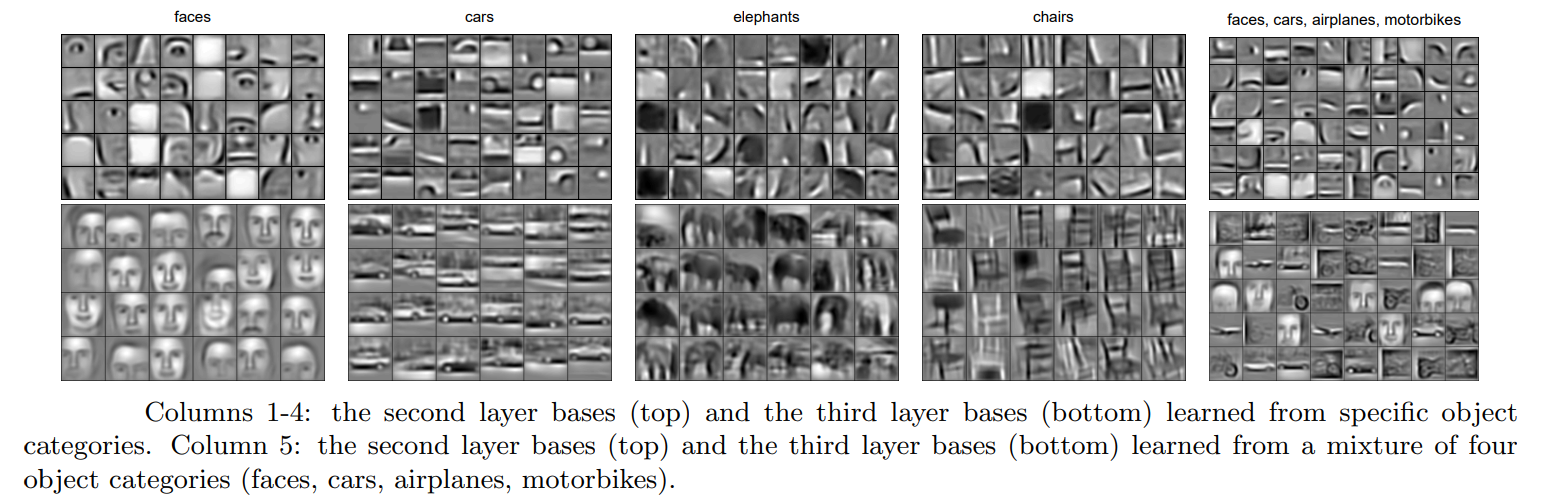 Figure 3: What convolutional filters learn to identify. Source: Convolutional Deep Belief Networks for Scalable Unsupervised Learning of Hierarchical Representations
A convolution layer has a set of learnable filters that act on small regions in the input to produce a representative output value for each region. For example, a 3x3 filter operates over a 3x3 size region and produces a value representative of the region. The repeated application of a filter over input regions produces an output which becomes the input to the next layer in the stack. Intuitively, the layers higher up get to "see" a larger region of the input. For example, a 3x3 filter in the second convolution layer operates on the output of the first convolution layer where each cell contains information about the 3x3 sized region in the input. If we assume a convolution operation with stride=1, then the filter in the second layer will "see'' the 5x5 sized region of the original input. This is called the receptive field of the convolution. The repeated application of convolutional layers progressively reduces the spatial dimensions of the input image and increases the field of vision of the filters which enables them to "see" complex shapes. Figure 4 shows the processing of a 1-D input by a convolution network. An element in the output layer is a representative of a relatively larger input chunk.
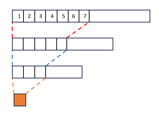 Figure 4: Receptive field of a 1d convolution with kernel size=3, applied 3 times. Assume stride=1 and no padding. After the 3rd successive application of the convolutional kernel, a single pixel is able to see 7 pixels in the original input image. Source: Author(s)
Once a convolutional layer can detect these objects and is able to generate their representations, we can use these representations for image classification, image segmentation, and object detection and localization. Broadly speaking, CNNs adhere to the following general principles:
- A Convolution layer either keeps the number of output channels © intact or doubles them.
- It keeps the spatial dimensions intact using a stride=1 or reduces them to a half using stride=2.
- It's common to pool the output of a convolution block to change the spatial dimensions of an image.
A convolution layer applies the kernel independently to each input. This could cause its output to vary for different inputs. A Batch Normalization layer typically follows a convolution layer to address this problem. Let's understand its role in detail in the next section.
Batch Normalization
Batch Normalization layer normalizes the channel values in the batch input to have a zero mean and a unit variance. This normalization is performed independently for each channel in the batch to ensure that the channel values for the inputs have the same distribution. Batch Normalization has the following benefits:
- It stabilizes the training process by preventing the gradients from becoming too small.
- It achieves faster convergence on our tasks.
If all we had was a stack of convolution layers, it would essentially be equivalent to a single convolution layer network because of the cascading effect of linear transformations. In other words, a sequence of linear transformations can be replaced with a single linear transformation which has the same effect. Intuitively, if we multiply a vector with a constant k₁ followed by multiplication with another constant k₂ , it is equivalent to a single multiplication by a constant k₁k₂. Hence, for the networks to be realistically deep, they must have a non-linearity to prevent their collapse. We will discuss ReLU in the next section which is frequently used as a non-linearity.
ReLU
ReLU is a simple non-linear activation function which clips the lowest input values to be greater than or equal to 0. It also helps with the vanishing gradients problem limiting the outputs to be greater than or equal to 0. The ReLU layer is typically followed by a pooling layer to shrink the spatial dimensions in the downscaling subnetwork or an un-pooling layer to bump the spatial dimensions in the upscaling subnetwork. The details are provided in the next section.
Pooling
A pooling layer is used to shrink the spatial dimensions of our inputs. Pooling with stride=2 will transform an input with spatial dimensions (H, W) to (H/2, W/2). Max-pooling is the most commonly used pooling technique in deep CNNs. It projects the maximum value in a grid of (say) 2x2 onto the output. Then, we slide the 2x2 pooling window to the next section based on the stride similar to convolutions. Doing this repeatedly with a stride=2 results in an output that is half the height and half the width of the input. Another commonly used pooling layer is the average-pooling layer, which computes the average instead of the max.
The reverse of a pooling layer is called an un-pooling layer. It takes an (H, W) dimension input and converts it into a (2H, 2W) dimension output for stride=2. A necessary ingredient of this transformation is selecting the location in the 2x2 section of the output to project the input value. To do this, we need a max-unpooling-index-map which tells us the target locations in the output section. This unpooling-map is produced by a previous max-pooling operation. Figure 5 shows examples of pooling and un-pooling operations.
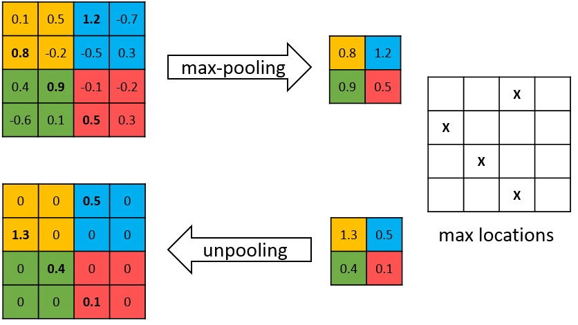 Figure 5: Max pooling and un-pooling. Source: DeepPainter: Painter Classification Using Deep Convolutional Autoencoders
We can consider max-pooling as a type of non-linear activation function. However, it's reported that using it to replace a non-linearity such as ReLU affects the network's performance. In contrast, average pooling can not be considered as a nonlinear function since it uses all its inputs to produce an output that is a linear combination of its inputs.
This covers all the basic building blocks of deep CNNs. Now, let's put them together to create a model. The model we have chosen for this exercise is called a SegNet. We'll discuss it next.
SegNet: A CNN-based model
SegNet is a deep CNN model based on the fundamental blocks that we have discussed in this article. It has two distinct sections. The bottom section, also called an encoder, down-samples the input to generate features representative of the input. The top decoder section up-samples the features to create per-pixel classification. Each section is composed of a sequence of Conv-BN-ReLU blocks. These blocks also incorporate pooling or un-pooling layers in downsampling and upsampling paths respectively. Figure 6 shows the arrangement of the layers in more detail. SegNet uses the pooling indices from the max-pooling operation in the encoder to determine which values to copy over during the max-unpooling operation in the decoder. While each element of an activation tensor is 4-bytes (32-bits), an offset within a 2x2 square can be stored using just 2-bits. This is more efficient in terms of memory used since these activations (or indices in the case of SegNet) need to be stored while the model runs.
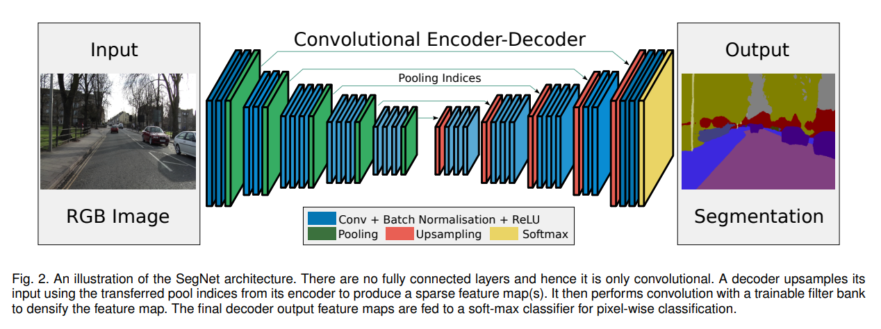 Figure 6: The SegNet model architecture for image segmentation. Source: SegNet: A Deep Convolutional Encoder-Decoder Architecture for Image Segmentation
This notebook contains all the code for this section.
This model has 15.27M trainable parameters.
The following configuration was used during model training and validation.
- The random horizontal flip and color jitter data augmentations are applied to the training set to prevent overfitting
- The images are resized to 128x128 pixels in a non-aspect preserving resize operation
- No input normalization is applied to the images; instead a batch normalization layer is used as the first layer of the model
- The model is trained for 20 epochs using the Adam optimizer with a LR of 0.001 and a StepLR Scheduler that decays the learning rate by 0.7 every 7 epochs
- The cross-entropy loss function is used to classify a pixel as belonging to a pet, the background, or a pet border
The model achieved a validation accuracy of 88.28% after 20 training epochs.
We plotted a gif showing how the model is learning to predict the segmentation masks for 21 images in the validation set.
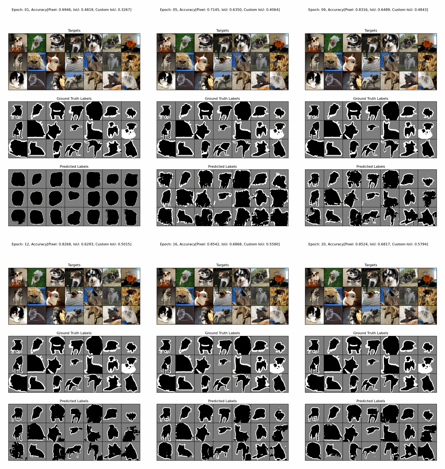 Figure 6: A gif showing how the SegNet model is learning to predict segmentation masks for 21 images in the validation set. Source: Author(s)
The definitions of all the validation metrics are described in Part-1 of this series.
If you'd like to see a fully-convolutional model for segmenting pet images implemented using Tensorflow, please see Chapter-4: Efficient Architectures of the Efficient Deep Learning Book.
Observations from model learning
Based on the development of the predictions that the trained model makes after every epoch, we can observe the following.
- The model is able to learn enough to make the output look in the right ballpark of the pet in the image even as early as 1 training epoch
- The border pixels are harder to segment since we're using an unweighted loss function that treats each success (or failure) equally, so getting the border pixels wrong doesn't cost the model much in terms of the loss. We would encourage you to investigate this and check what strategies you could try to fix this issue. Try using Focal Loss and see how it performs
- The model seems to be learning even after 20 training epochs. This suggests that we could improve validation accuracy if we trained the model longer
- Some of the ground-truth labels themselves are hard to figure out - for example, the mask of the dog in the middle row, last column has a lot of unknown pixels in the area where the body of the dog is occluded by plants. This is very hard for the model to figure out, so one should always expect loss in accuracy for such examples. However, this doesn't mean that the model isn't doing well. One should always spot check the predictions to develop a sense of the model's behavior in addition to looking at the overall validation metrics.
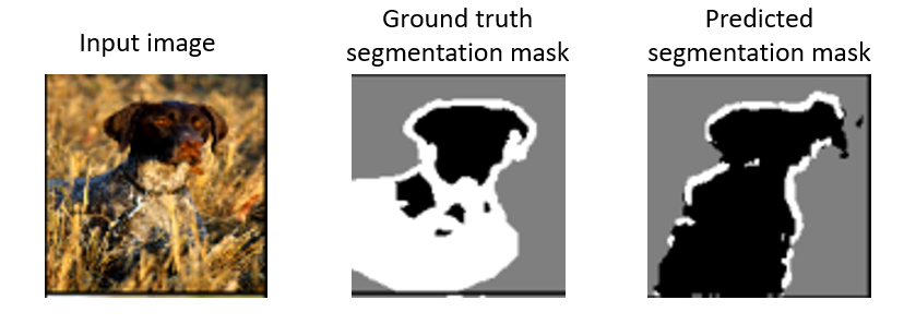 Figure 7: An example of the ground truth segmentation mask containing a lot of unknown pixels. This is a very hard input for any ML model. Source: Author(s)
Conclusion
In part-2 of this series, we learned about the basic building blocks of deep CNNs for vision AI. We saw how to implement the SegNet model from scratch in PyTorch, and we visualized how the model trained on successive epochs performs on 21 validation images. This should help you appreciate how quickly models can learn enough to make the output look somewhere in the right ballpark. In this case, we can see segmentation masks that roughly resemble the actual segmentation mask as early as the first training epoch!
In the next part of this series, we'll take a look at how we can optimize our model for on-device inference and reduce the number of trainable parameters (and hence model size) while keeping the validation accuracy roughly the same.
Further Reading
Read more about convolutions here:
- The course titled "Ancient Secrets of computer vision" at The University of Washington taught by Joseph Redmon has an excellent set of videos on Convolutions (especially chapters 4, 5, and 13), which we highly recommend watching
- A guide to convolution arithmetic for deep learning (highly recommended)
- https://towardsdatascience.com/computer-vision-convolution-basics-2d0ae3b79346
- The Conv2d layer in PyTorch (documentation)
- What do convolutions learn?
- Convolution visualizer
Read more about batch normalization here:
- Batch normalization: Wikipedia
- Batch normalization: Machine learning mastery
- BatchNorm2d layer in PyTorch here.
Read more about activation functions and ReLU here:
- ReLU: Machine learning mastery
- ReLU: Wikipedia
- ReLU: Quora
- ReLU API in PyTorch
Register Now to Continue Reading
Unlock Towards Data Science with a Free Account
All articles on Towards Data Science are available to registered users. Create a free account today to access this article and thousands more.
Register for freeSign in to your account
 Written By
See all from Dhruv Matani
CnnConvolutional NetworkDeep LearningPytorchPytorch Image Segment
Share This Article
Towards Data Science is a community publication. Submit your insights to reach our global audience and earn through the TDS Author Payment Program.
Write for TDS
Related Articles
Deep Learning
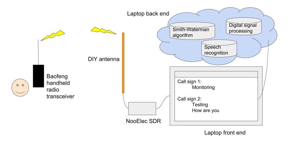
A project on building a speech recognition system for amateur radio communication.
Chris
October 6, 20183 min read
Artificial Intelligence
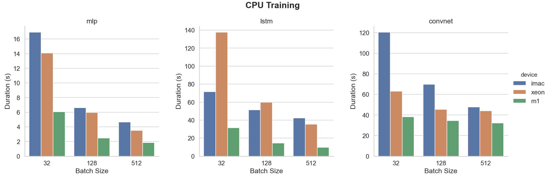
Compare Apple Silicon M1 CPU and GPU performances to high-end configurations on MLP, CNN and LSTM models
Fabrice Daniel
December 26, 20206 min read
Artificial Intelligence
If you are searching for a way to organize, manage and log the steps and operations during a training process and don't want to use PyTorch...
Tudor Surdoiu
October 4, 20224 min read
Artificial Intelligence
Leverage Bayesian Theory to boost your performance
Nikos Kafritsas
June 8, 20222 min read
Artificial Intelligence
Fourth CNN?
Vidisha Jitani
October 6, 20204 min read
Deep Learning
Artificial intelligence software was used to enhance the grammar, flow, and readability of this article's text.
Anthony Alcaraz
December 3, 20239 min read
Deep Learning
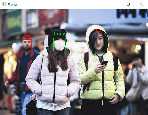
COVID-19: Tutorial on how to build a face mask detector using YOLOv3. *For inference, both video streams and images can be used.
Stefanos Kanellopoulos
April 12, 20219 min read
Artificial Intelligence
Analyze and Visualize Artists and Artworks Metadata
Margaret Maynard-Reid
November 23, 20203 min read
Artificial Intelligence
Code and Theory
Alexey Kravets
July 24, 20237 min read
Your home for data science and AI. The world's leading publication for data science, data analytics, data engineering, machine learning, and artificial intelligence professionals.
Subscribe to Our NewsletterWrite For TDS•About•Advertise•Privacy Policy•Terms of Use
© Insight Media Group, LLC 2026•The New Stack•roadmap.sh•Creator Network
Recommended Articles
Close