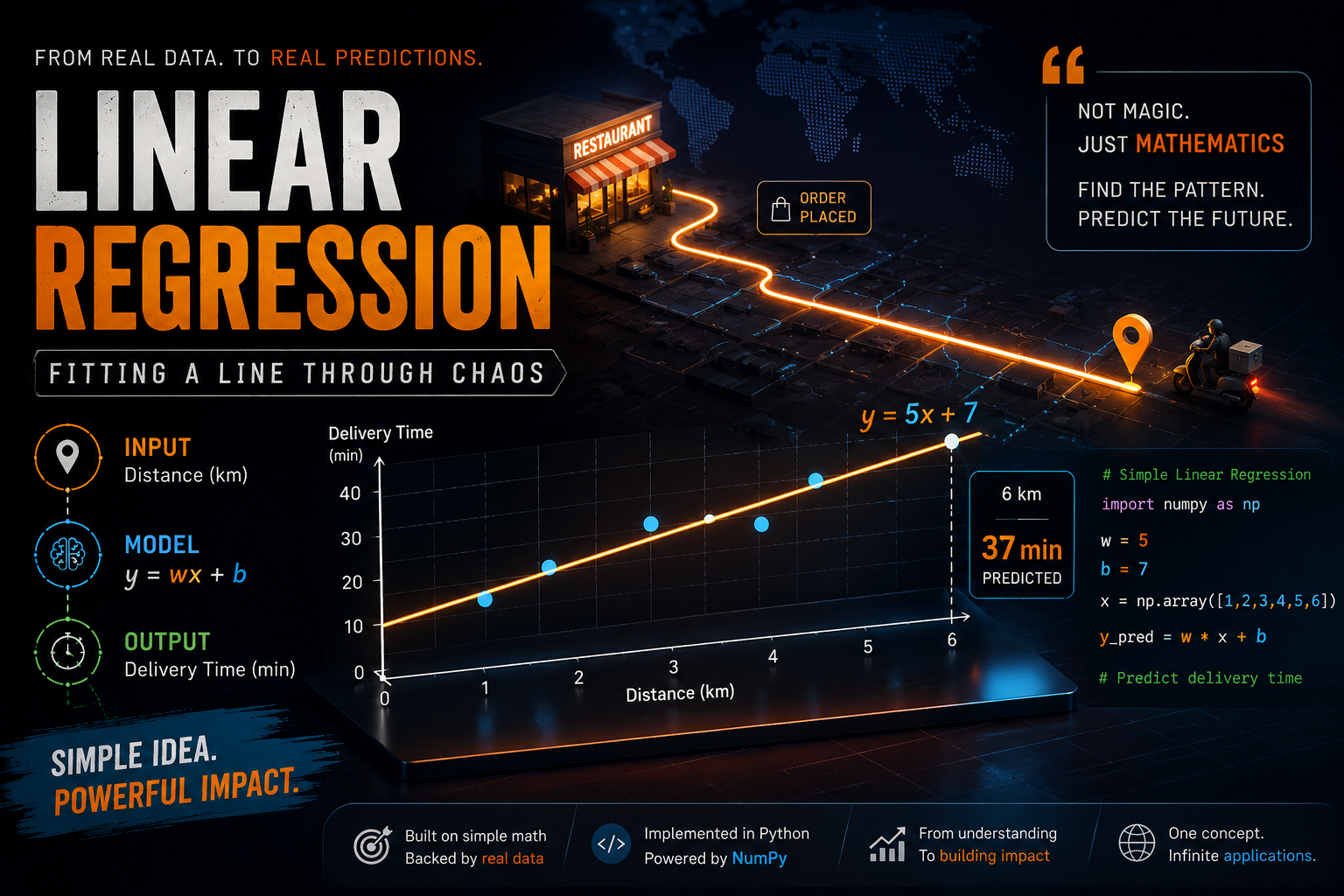
A few days ago, I ordered food from an app, and right after placing the order, it showed: "Arriving in 32 minutes." The delivery boy hadn't even picked up the order yet. He hadn't even started riding. But the app was already confident enough to give me an exact number.
That number wasn't pulled out of thin air. Somewhere behind that app, there's a model doing exactly what we talked about in the last post, looking at some inputs, and predicting an output. In this post, we're going to build the simplest possible version of that idea ourselves, with real numbers and a little bit of actual code.
Let's stick with the delivery example, but simplify it down to just one input: distance.
If you had to guess how long a delivery takes, using only the distance in kilometers, what would your guess depend on? Probably two things. First, how far the food has to travel, more distance should mean more time. Second, some baseline time that exists no matter what, the time it takes to pack the order, hand it to the rider, and get the bike moving, even before a single kilometer is covered.
Linear regression uses a formula to capture this:
prediction = w × x + b
Here's what each piece actually means, in plain terms:
x is the input we already know. In our case, the distance in kilometers.
w is called the weight. It tells us how much the prediction changes for every extra kilometer. If w is 5, every additional kilometer adds 5 minutes to the prediction. If you've seen the equation of a line before, this is just the slope.
b is called the bias. It's the starting point, roughly, the time we'd predict at zero distance. Packing the order, handing it over, getting the bike out of the parking area, all of that lives inside b. In line terms, this is the intercept.
Weight and bias, slope and intercept, same idea, different vocabulary depending on which room you're standing in. ML people say weight and bias. Math people say slope and intercept. Worth filing away, because you'll run into both.
So the formula is really just saying: start with a base time (b), then add a little more time for every kilometer of distance (w × x).
One clarification before we go further: this equation, w × x + b, is the model. It's the shape of the guess. Linear regression itself is the process of figuring out which w and b make that shape actually fit your data well. We haven't done that part yet. Right now we're just going to eyeball it.
Suppose we look at five past orders and their actual delivery times:
Distance (km)	    Actual Delivery Time (min)
    1	                      13
    2	                      16
    3	                      23
    4	                      26
    5                         34
Look at this table for a second before reading further. Notice anything?
It's roughly a straight line, but not exactly. Going from 1km to 2km only adds 3 minutes. Going from 2km to 3km adds 7. It's not a clean staircase. If you squint, though, the overall trend still climbs at something like 5 minutes per kilometer, with a starting point somewhere around 7 or 8 minutes.
This is actually closer to how real data behaves. Nothing about delivery times is going to line up perfectly: traffic, how busy the kitchen was, whether the rider hit every light red. That variation is what's usually called noise: the bumps in the data that don't come from distance at all, but from everything else going on around it. There's no single line that touches all five points exactly. What we're really looking for is a line that gets close to all of them, even if it doesn't nail any single one.
Here's a scatter of those five points, with a rough straight line drawn through them:
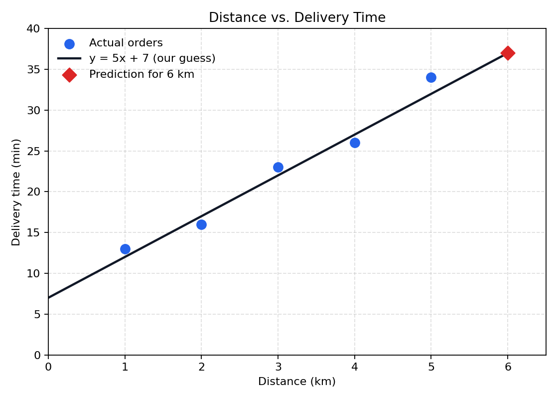
The line doesn't pass through every point, and that's fine; it's not supposed to. It's just supposed to capture the trend.
So let's put a number on that trend. Looking at the table, the slope looks like it's somewhere around 5 minutes per kilometer, and the line looks like it would cross zero distance somewhere around 7 or 8 minutes. Nothing rigorous, just eyeballing it. Let's go with w = 5, b = 7 as a rough first guess and see how it holds up. Could a different pair of numbers fit these five points slightly better? Probably. That question, how do you find the best w and b, not just a decent one, is exactly what we're building toward.
Let's check how our guess does for a distance of 3 km:
prediction = w × x + b
prediction = 5 × 3 + 7
prediction = 15 + 7
prediction = 22 minutes
The actual value in the table was 23. Close, but not a match. That one minute gap is the model being wrong by a little, and that's fine. It's actually the whole point: we're not looking for a formula that memorizes the table, we're looking for one that captures the general pattern well enough to be useful.
We can even write that gap down as a number:
error = prediction - actual
error = 22 - 23
error = -1 minute
We were off by one minute on this one. Nothing more to do with that number yet; just notice that every row in the table would give us a slightly different error, and we're going to need a way to turn all five of those into a single verdict on how good our line is. Hold that thought.
Now here's the real test, what would this formula predict for a distance it has never seen before, say 6 km?
prediction = 5 × 6 + 7
prediction = 30 + 7
prediction = 37 minutes
Nobody told the formula the answer for 6 km. We reused the same w and b we roughly guessed from the pattern, and it gave us an estimate based on that pattern. Whether 37 minutes is actually a good estimate isn't something we can say yet, we don't have a real 6 km order to check it against, and right now we don't even have a solid way to measure "good." That's the idea we're building toward: a trained model shouldn't memorize the table, it should capture the pattern behind the data and reuse that pattern on new inputs. We're not there yet. We just picked numbers that looked about right.
Quick side note on b: don't read too much into "7 minutes at 0 km" as a literal real-world fact. A delivery of zero distance isn't really a thing that happens. b is just where the line crosses the y-axis mathematically, a baseline the model implies, not a guarantee that any real order takes exactly 7 minutes.
We just picked w and b by looking at a small table and estimating. That won't work on a real dataset with thousands of noisy orders, we'll fix that in the next two posts. But to be clear about what we actually did here: we chose w and b ourselves. Nothing was trained. The model didn't learn anything yet, we handed it the answer. Actually training it, so it finds w and b on its own, is what the next two posts are about.
For now, let's take the w and b we picked, and write actual code that does the same math.
Here's the plain, no-shortcuts version first:
def predict(x, w, b):
    return w * x + b

# the values we picked by eye
w = 5
b = 7

# a list of distances we want predictions for
distances = [1, 2, 3, 4, 5, 6]

# predicting one by one, using a normal loop
predictions = []
for x in distances:
    predictions.append(predict(x, w, b))

print(predictions)
# [12, 17, 22, 27, 32, 37]
There's nothing hidden inside predict(). It's literally the equation we just wrote out by hand, typed into Python.
This works fine, and honestly, for six numbers, a loop is perfectly readable. But real datasets don't have six rows, they have thousands or even millions. Running a Python loop over a million rows, one at a time, adds up. This is where a library called NumPy comes in, it lets us do the exact same calculation on an entire list of numbers at once, without writing a loop ourselves.
import numpy as np

distances = np.array([1, 2, 3, 4, 5, 6])
w = 5
b = 7

predictions = w * distances + b

print(predictions)
# [12 17 22 27 32 37]
Same formula, same result. NumPy just lets us apply the operation to the whole array at once instead of looping through it ourselves; this is called vectorization, and it starts to matter once "six numbers" turns into a real dataset. We'll lean on this style for the rest of the series, so it's worth getting comfortable with it early.
Quick recap before we move on:
A linear model: y = wx + b w
controls how much the prediction changes as x increases, the slope
b is the baseline/intercept, the value the line implies at x = 0
We used the model to predict a distance it had never seen (6 km)
We picked w and b ourselves, by eye, nothing was actually trained
The model didn't perfectly match the data, and that's expected, not a bug
We cheated a bit in this post. We only landed on w = 5 and b = 7 because we stared at a small table and made a reasonable guess. It got close, not exact. Real data is messier than five rows, and no amount of staring at a spreadsheet is going to hand you the right w and b when you've got thousands of them.
So how does a machine find the right w and b on its own, without a human eyeballing anything?
That's exactly what the next two posts are about. First, we need a way to measure exactly how wrong a given w and b are, that's called the cost function. Then, we need a way for the machine to use that measurement to automatically improve its guess, step by step, that's gradient descent. Put those two together, and you've got the core mechanism a machine uses to find its own w and b, on data far messier than our little table.
The full code from this post, along with the dataset, is up on GitHub here: https://github.com/tharun-pandya/Machine-Learning-Blog-Series/blob/main/Linear_Regression.ipynb
See you in the next one.