保留正文与补采附件。源页面当前未重新核验;具体限制见交付清单。
 We value your privacy
We use cookies to enhance your browsing experience, serve personalised ads or content, and analyse our traffic. By clicking "Accept All", you consent to our use of cookies.
Customise Reject All Accept All
Customise Consent Preferences
 We use cookies to help you navigate efficiently and perform certain functions. You will find detailed information about all cookies under each consent category below.
The cookies that are categorised as "Necessary" are stored on your browser as they are essential for enabling the basic functionalities of the site. ... Show more
NecessaryAlways Active
Necessary cookies are required to enable the basic features of this site, such as providing secure log-in or adjusting your consent preferences. These cookies do not store any personally identifiable data.
-
Cookie
BCTempID
-
Duration
10 minutes
-
Description
No description available.
-
Cookie
__cf_bm
-
Duration
1 hour
-
Description
This cookie, set by Cloudflare, is used to support Cloudflare Bot Management.
-
Cookie
AWSALBCORS
-
Duration
7 days
-
Description
Amazon Web Services set this cookie for load balancing.
-
Cookie
_cfuvid
-
Duration
session
-
Description
Cloudflare sets this cookie to track users across sessions to optimize user experience by maintaining session consistency and providing personalized services
-
Cookie
li_gc
-
Duration
6 months
-
Description
Linkedin set this cookie for storing visitor's consent regarding using cookies for non-essential purposes.
-
Cookie
__hssrc
-
Duration
session
-
Description
This cookie is set by Hubspot whenever it changes the session cookie. The __hssrc cookie set to 1 indicates that the user has restarted the browser, and if the cookie does not exist, it is assumed to be a new session.
-
Cookie
__hssc
-
Duration
1 hour
-
Description
HubSpot sets this cookie to keep track of sessions and to determine if HubSpot should increment the session number and timestamps in the __hstc cookie.
-
Cookie
wpEmojiSettingsSupports
-
Duration
session
-
Description
WordPress sets this cookie when a user interacts with emojis on a WordPress site. It helps determine if the user's browser can display emojis properly.
-
Cookie
BCSessionID
-
Duration
1 year 1 month 4 days
-
Description
Blueconic sets this cookie as a unique identifier for the BlueConic profile.
-
Cookie
_octo
-
Duration
1 year
-
Description
No description available.
-
Cookie
logged_in
-
Duration
1 year
-
Description
No description available.
-
Cookie
__Secure-YEC
-
Duration
past
-
Description
YouTube sets this cookie to stores the user's video player preferences using embedded YouTube video
-
Cookie
__eoi
-
Duration
6 months
-
Description
Description is currently not available.
-
Cookie
AWSALBTGCORS
-
Duration
7 days
-
Description
No description available.
-
Cookie
login-status-p
-
Duration
past
-
Description
Description is currently not available.
-
Cookie
AWSALBTG
-
Duration
7 days
-
Description
No description available.
-
Cookie
csrf_token
-
Duration
session
-
Description
No description available.
-
Cookie
token_v2
-
Duration
1 day
-
Description
Description is currently not available.
-
Cookie
D
-
Duration
1 year
-
Description
Description is currently not available.
-
Cookie
PHPSESSID
-
Duration
session
-
Description
This cookie is native to PHP applications. The cookie stores and identifies a user's unique session ID to manage user sessions on the website. The cookie is a session cookie and will be deleted when all the browser windows are closed.
-
Cookie
VISITOR_PRIVACY_METADATA
-
Duration
6 months
-
Description
YouTube sets this cookie to store the user's cookie consent state for the current domain.
-
Cookie
cookietest
-
Duration
session
-
Description
The cookietest cookie is typically used to determine whether the user's browser accepts cookies, essential for website functionality and user experience.
-
Cookie
__Host-airtable-session
-
Duration
1 year
-
Description
This cookie is used to enable us to integrate the services of Airtable.
-
Cookie
__Host-airtable-session.sig
-
Duration
1 year
-
Description
This cookie is used to enable us to integrate the services of Airtable.
-
Cookie
m
-
Duration
1 year 1 month 4 days
-
Description
Stripe sets this cookie for fraud prevention purposes. It identifies the device used to access the website, allowing the website to be formatted accordingly.
-
Cookie
BIGipServer*
-
Duration
session
-
Description
Marketo sets this cookie to collect information about the user's online activity and build a profile about their interests to provide advertisements relevant to the user.
-
Cookie
__cfruid
-
Duration
session
-
Description
Cloudflare sets this cookie to identify trusted web traffic.
-
Cookie
_GRECAPTCHA
-
Duration
6 months
-
Description
Google Recaptcha service sets this cookie to identify bots to protect the website against malicious spam attacks.
-
Cookie
__Secure-YNID
-
Duration
6 months
-
Description
Google cookie used to protect user security and prevent fraud, especially during the login process.
-
Cookie
cookieyes-consent
-
Duration
1 year
-
Description
CookieYes sets this cookie to remember users' consent preferences so that their preferences are respected on subsequent visits to this site. It does not collect or store any personal information about the site visitors.
Functional
Functional cookies help perform certain functionalities like sharing the content of the website on social media platforms, collecting feedback, and other third-party features.
-
Cookie
lidc
-
Duration
1 day
-
Description
LinkedIn sets the lidc cookie to facilitate data center selection.
-
Cookie
brw
-
Duration
1 year
-
Description
No description available.
-
Cookie
brwConsent
-
Duration
5 minutes
-
Description
Description is currently not available.
-
Cookie
WMF-Uniq
-
Duration
1 year
-
Description
Description is currently not available.
-
Cookie
loom_anon_comment
-
Duration
1 year
-
Description
No description available.
-
Cookie
loom_referral_video
-
Duration
session
-
Description
Description is currently not available.
-
Cookie
VISITOR_INFO1_LIVE
-
Duration
6 months
-
Description
A cookie set by YouTube to measure bandwidth that determines whether the user gets the new or old player interface.
-
Cookie
yt-remote-connected-devices
-
Duration
Never Expires
-
Description
YouTube sets this cookie to store the user's video preferences using embedded YouTube videos.
-
Cookie
ytidb::LAST_RESULT_ENTRY_KEY
-
Duration
Never Expires
-
Description
The cookie ytidb::LAST_RESULT_ENTRY_KEY is used by YouTube to store the last search result entry that was clicked by the user. This information is used to improve the user experience by providing more relevant search results in the future.
-
Cookie
yt-remote-device-id
-
Duration
Never Expires
-
Description
YouTube sets this cookie to store the user's video preferences using embedded YouTube videos.
-
Cookie
yt-remote-session-name
-
Duration
session
-
Description
The yt-remote-session-name cookie is used by YouTube to store the user's video player preferences using embedded YouTube video.
-
Cookie
yt-remote-fast-check-period
-
Duration
session
-
Description
The yt-remote-fast-check-period cookie is used by YouTube to store the user's video player preferences for embedded YouTube videos.
-
Cookie
yt-remote-session-app
-
Duration
session
-
Description
The yt-remote-session-app cookie is used by YouTube to store user preferences and information about the interface of the embedded YouTube video player.
-
Cookie
yt-remote-cast-available
-
Duration
session
-
Description
The yt-remote-cast-available cookie is used to store the user's preferences regarding whether casting is available on their YouTube video player.
-
Cookie
yt-remote-cast-installed
-
Duration
session
-
Description
The yt-remote-cast-installed cookie is used to store the user's video player preferences using embedded YouTube video.
-
Cookie
cp_session
-
Duration
3 months
-
Description
Codepen sets this cookie for Help systems found in the website.
-
Cookie
loid
-
Duration
1 year 1 month 4 days
-
Description
This cookie is set by the Reddit. The cookie enables the sharing of content from the website onto the social media platform.
Analytics
Analytical cookies are used to understand how visitors interact with the website. These cookies help provide information on metrics such as the number of visitors, bounce rate, traffic source, etc.
-
Cookie
__hstc
-
Duration
6 months
-
Description
Hubspot set this main cookie for tracking visitors. It contains the domain, initial timestamp (first visit), last timestamp (last visit), current timestamp (this visit), and session number (increments for each subsequent session).
-
Cookie
hubspotutk
-
Duration
6 months
-
Description
HubSpot sets this cookie to keep track of the visitors to the website. This cookie is passed to HubSpot on form submission and used when deduplicating contacts.
-
Cookie
_ga
-
Duration
1 year 1 month 4 days
-
Description
Google Analytics sets this cookie to calculate visitor, session and campaign data and track site usage for the site's analytics report. The cookie stores information anonymously and assigns a randomly generated number to recognise unique visitors.
-
Cookie
ga*
-
Duration
1 year 1 month 4 days
-
Description
Google Analytics sets this cookie to store and count page views.
-
Cookie
__Host-psifi.analyticsTrace
-
Duration
6 hours
-
Description
Description is currently not available.
-
Cookie
__Host-psifi.analyticsTraceV2
-
Duration
6 hours
-
Description
Description is currently not available.
-
Cookie
_gh_sess
-
Duration
session
-
Description
GitHub sets this cookie for temporary application and framework state between pages like what step the user is on in a multiple step form.
-
Cookie
YSC
-
Duration
session
-
Description
YSC cookie is set by Youtube and is used to track the views of embedded videos on Youtube pages.
-
Cookie
ajs_anonymous_id
-
Duration
1 year
-
Description
This cookie is set by Segment to count the number of people who visit a certain site by tracking if they have visited before.
-
Cookie
vuid
-
Duration
1 year 1 month 4 days
-
Description
Vimeo installs this cookie to collect tracking information by setting a unique ID to embed videos on the website.
Performance
Performance cookies are used to understand and analyse the key performance indexes of the website which helps in delivering a better user experience for the visitors.
-
Cookie
AWSALB
-
Duration
7 days
-
Description
AWSALB is an application load balancer cookie set by Amazon Web Services to map the session to the target.
-
Cookie
acq
-
Duration
past
-
Description
Description is currently not available.
-
Cookie
acq.sig
-
Duration
past
-
Description
Description is currently not available.
-
Cookie
ptc
-
Duration
2 years
-
Description
No description available.
Advertisement
Advertisement cookies are used to provide visitors with customised advertisements based on the pages you visited previously and to analyse the effectiveness of the ad campaigns.
-
Cookie
muc_ads
-
Duration
1 year 1 month 4 days
-
Description
Twitter sets this cookie to collect user behaviour and interaction data to optimize the website.
-
Cookie
guest_id_marketing
-
Duration
1 year 1 month 4 days
-
Description
Twitter sets this cookie to identify and track the website visitor.
-
Cookie
guest_id_ads
-
Duration
1 year 1 month 4 days
-
Description
Twitter sets this cookie to identify and track the website visitor.
-
Cookie
personalization_id
-
Duration
1 year 1 month 4 days
-
Description
Twitter sets this cookie to integrate and share features for social media and also store information about how the user uses the website, for tracking and targeting.
-
Cookie
guest_id
-
Duration
1 year 1 month 4 days
-
Description
Twitter sets this cookie to identify and track the website visitor. It registers if a user is signed in to the Twitter platform and collects information about ad preferences.
-
Cookie
bcookie
-
Duration
1 year
-
Description
LinkedIn sets this cookie from LinkedIn share buttons and ad tags to recognize browser IDs.
-
Cookie
__Secure-ROLLOUT_TOKEN
-
Duration
6 months
-
Description
YouTube sets this cookie to manage feature rollout and experimentation. It helps Google control which new features or interface changes are shown to users as part of testing and staged rollouts, ensuring consistent experience for a given user during an experiment.
-
Cookie
yt.innertube::nextId
-
Duration
Never Expires
-
Description
YouTube sets this cookie to register a unique ID to store data on what videos from YouTube the user has seen.
-
Cookie
yt.innertube::requests
-
Duration
Never Expires
-
Description
YouTube sets this cookie to register a unique ID to store data on what videos from YouTube the user has seen.
-
Cookie
session_tracker
-
Duration
session
-
Description
This cookie is set by the Reddit. This cookie is used to identify trusted web traffic. It also helps in adverstising on the website.
-
Cookie
edgebucket
-
Duration
session
-
Description
Reddit sets this cookie to save the information about a log-on Reddit user, for the purpose of advertisement recommendations and updating the content.
-
Cookie
did
-
Duration
1 year
-
Description
Arbor sets this cookie to show targeted ads to site visitors.This cookie expires after 2 months or 1 year.
Uncategorised
Other uncategorised cookies are those that are being analysed and have not been classified into a category as yet.
No cookies to display.
Reject All Save My Preferences Accept All
Toggle SearchToggle Mobile Navigation
Publish AI, ML & data-science insights to a global community of data professionals.
Sign inSubmit an Article
LatestEditor's PicksNewsletterShipAI
Write For TDS
LinkedInXToggle Search
Data Science
Multivariant Linear Regression
Oh boy, homoscedasticity!
James Andrew Godwin
March 12, 202111 min read
Oh boy, homoscedasticity
 Multivariant Regression | Photo by Paweł Czerwiński
This article is a continuation of my previous one on Linear Regression.
It is important to reiterate from my last article about the error formulae in least-squares regression.
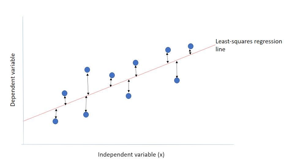 Least-squares regression selects the line with the lowest total SSE
The sum of this sum of squares error here is the discrepancy between the theoretical value on the line and the actual observed value, which is the point which is the blue dots. Those discrepancies squared and then sum up those squares that hold total area is the SSE , sum of squared error.
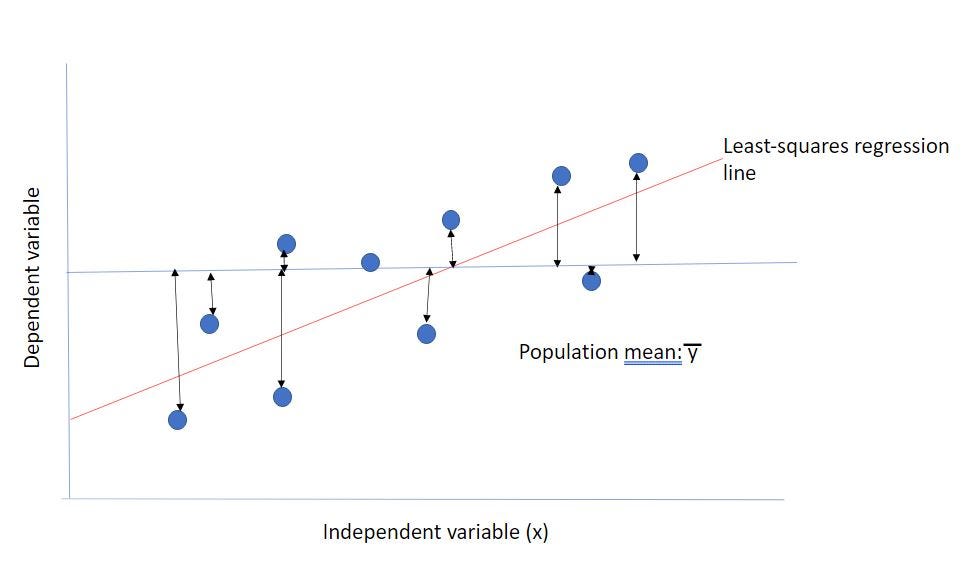 Sum of Squares Regression (SSR)
Here is the sum of squares regression (SSR). This basically says how much variance there is; what is basically the amount of effect that we see between the predictive values, how much the model has to do. If this is a very large number, it does not by itself mean that the model is good or bad. But if this SSR is substantially larger than it, or the sum of squares of the regression is substantially larger than the sum of squares of these discrepancies (SSE), then it is a good model. The measurement is between the predicted values and the mean.
The sum of squares total (SST)is sometimes equal to SSR + SSE. The primary sometimes is if you use the least-squares regression, to begin with, which sort of makes sense - we are summing up squares here so you are doing a least-squares regression. And the other more important thing is, and this is the one that people forget all the time, is that this equation, SST = SSR +SSE is only true for the training data. It is not true for the test data. The reason why is the SSE can be arbitrarily large with test data. And if it gets too large then things can go wrong. SSE can get arbitrarily large, so even larger than SST, it can become a lot larger than SST. SST is based on only the training data while SSE is based on your test data.
 SSE can be bigger than SST
Therefore it is very possible to have a negative value for R². And as we all know, R² cannot be negative if it were truly a square of something. But as you see, this formula here is not a squaring of any Pearson's R or anything like that.
Another accuracy measure of the line is using the Root Mean Squared Error (RMSE). Using this as an estimate of the error means we are losing one more degree of freedom than the standard deviation, so we write the RSE as:
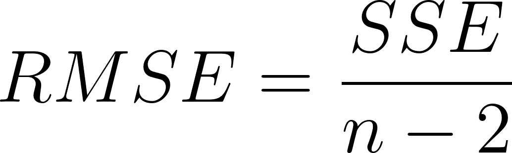 Defined in terms of SSE
text
# mean squared error
text
mse = np.sum((y_pred - y_actual)**2)
text
# root mean squared error, m is number of training samples
rmse = np.sqrt(mse/m)
# results.mse_resid
Assumptions
Here are some important assumptions of linear regression.
- Linear relationship between the dependent variable and independent variables
- Measurement error is random
- Residuals are homoscedastic
The primary assumption is residuals are homoscedastic. Homoscedasticity means that they are roughly the same throughout, which means your residuals do not suddenly get larger. And this is often not the case, often things are not homoscedastic. What do you do then? Well, if you can do one of those tricks, like changing the y values, transforming them before you do any linear regression, then great! Otherwise, what can be done when the assumption is not valid? This is the dirty secret: they do nothing. They just pretend that their residuals are homoscedastic in spite of the fact that they are heteroscedastic, which means that the error is not consistent throughout.
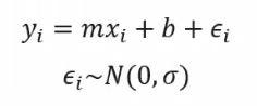 Our assumed homoscedastic model
N.B: The errors do not be normally distributed to be homoscedastic, the errors just need to be roughly the same throughout. They do need to be centered about zero, however.
Outliers
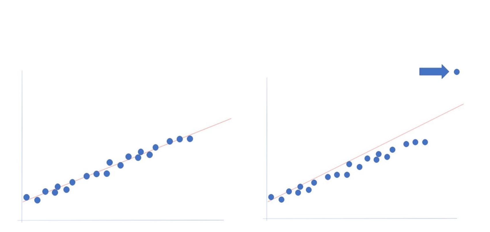 Susceptible to outliers: an outlier is an observation with a large residual
Linear regressions are susceptible to outliers. Here, you have a nice linear relationship, this line going through these data points perfectly. The second image is not because that one data point up in the top right is pulling the regression line way up there. Outliers like this can really be a problem, you can get rid of outliers and like that in a variety of ways, like leverage and Cook's Distance.
Linear regression fits a line based on the means of the x and y values. It fits a line that goes through the means of both values. This line pivots around the point relative to the pull of each point. Points that are farther away from the mean pull harder on the slope - this is leverage. Another way to quantify the 'pull' of each point, is to fit the line to the data without each point and see how the parameters move: this is Cook's Distance.
Coefficients and p-values
When the regression line is linear the regression coefficient is the constant that represents the rate of change of one variable as a function of the other - it is the slope of the regression line.
- The p-values for the coefficients indicate whether these relationships are statistically significant.
- The t statistic is the coefficient divided by its standard error.
Checking the residuals
This is important! You should always check for trends in the residuals.
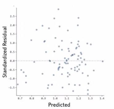 You should not see any pattern
There are more data points on the right than the left, and that is ok, that is just the shape of the data. The predicted values on the x-axis and the residuals, the error from the predicted value, on the y-axis.
- Residuals = Obsevered (actual data) - Predicted (where the data moves to the regression line)
Positive values for the residual (on the y-axis) indicate that the prediction was too low, and negative values indicate that the prediction was too high. A zero means that the guess was exactly correct!
THERE SHOULD BE NO PATTERN IN THE RESIDUALS!
The question is, are the residuals closer to this dotted line on the right-hand side than they are on the left-hand side overall? Or even worse - do you see more residuals beneath the dotted line than above the dotted line? What is the dotted line, the dotted line is zero where you have zero residual. The residual again is the discrepancy between your predicted y value and your actual y value. They should all hover around zero because well, the point of the fact of having a predicted y value was to explain your data. And the predicted y value should be generally close to your y value.
When this is not the case you have residuals. Sometimes, seeing an obvious trend in your residuals is an opportunity. That means that you can then use that trend in your residuals to add another model only to your residuals.
Always plot the residuals to check for trends. Check the residuals versus y, and make sure that they are, say, always positively correlated, the higher the correlation, the worse the fit. The reason is that if there is a high correlation to the residuals with y, that means that as y gets larger, your residuals get larger. And this actually happens a lot. Testing the normality of the residuals is also important.
A common sign that your residuals are heteroscedastic is the "fan-shaped" errors, whereby the errors are larger on the right-hand side than the left-hand side.
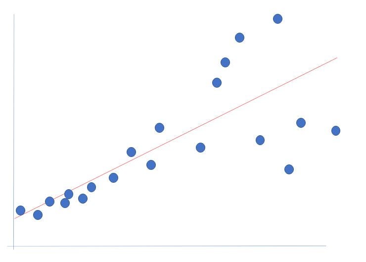 Note the "fan-shape" in the raw data, the errors are much larger on RHS than LHS
Again, there should be no trends apparent in the residuals. But oftentimes the residuals can be assumed to be homoscedastic when they are not, like the fan-shape below. The third outcome, the nonlinear one, is a really bad one that cannot be assumed to be homoscedastic, the error trend is parabolic.
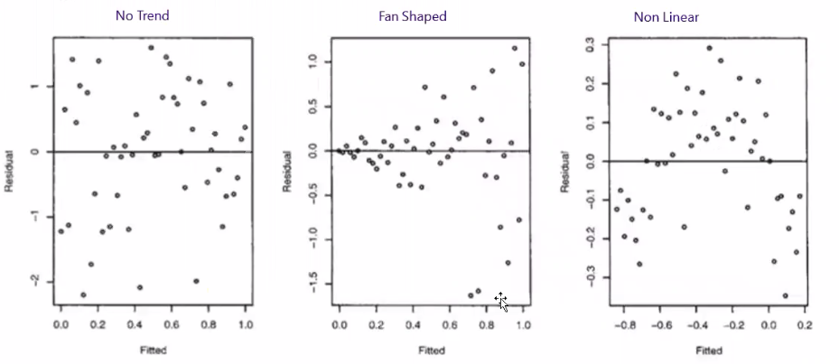 This nonlinear error trend is likely an indication that the data has a relationship that is not best captured with the parameters used; the residuals have information in them. It looks as if we could actually fit a polynomial to these residuals. Or we could simply add the polynomial to our linear model in the first place and overall we would have fewer errors after doing this.
Multiple linear regression
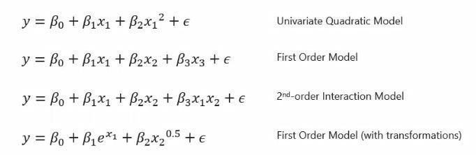 All these regressions are linear in parameters
As mentioned in my previous article, why not make the variables in the last formula linear by saying the exponent is a different variable, like z? These are the new variables that we then have a linear setup for and the equation becomes a multivariant linear regression.
 Multiple independent variables make this an example of multivariant linear regression
One hot encoding vs dummy variables
This is commonly misunderstood. There is one-hot encoding (OHE) as one way of doing things, then there is the dummy variable way of encoding for linear regression. The dummy variable is basically the same as OHE, you just do n-1 of the variables. Gender is not OHE when all you have is a column labeled "gender" with a 1 being "male" and a 0 being "female", this here is actually a dummy variable. This is not one hot encoding because there is no column for females, there is only a column for males. So the column should not be called gender, because there exists no such gender as one and zero, this column should be called is male.
With the dummy variable, you drop columns, with OHE you never drop columns. That is the definition of what one-hot encoding is. One hot encoding is not a data science term , rather it comes from a very different area of engineering. Imparting dummy variables is statistically more useful because you will not have colinearity. But you probably will not have colinearity anyway, probably not for certain. Using OHE allows for better model interpretation. Remember that with OHE, you never drop columns, doing so is imparting a dummy variable.
Multiple linear regression in python
With the following example, we want to predict the stock price index, just like everyone else.
N.B: For simplicity, and this is a big no-no, this model just uses the test data for fitting - there is no train/tune/test split.
text
# imports
from pandas import DataFrame
from sklearn import linear_model
import statsmodels.api as sm
from sklearn.metrics import mean_squared_error, r2_score
import matplotlib.pyplot as plt
text
# create dataframe from stock data
Stock_Market = {'Year': [2017,2017,2017,2017,2017,2017,2017,2017,2017,2017,2017,2017,2016,2016,2016,2016,2016,2016,2016,2016,2016,2016,2016,2016],
 'Month': [12, 11,10,9,8,7,6,5,4,3,2,1,12,11,10,9,8,7,6,5,4,3,2,1],
 'Interest_Rate': [2.75,2.5,2.5,2.5,2.5,2.5,2.5,2.25,2.25,2.25,2,2,2,1.75,1.75,1.75,1.75,1.75,1.75,1.75,1.75,1.75,1.75,1.75],
 'Unemployment_Rate': [5.3,5.3,5.3,5.3,5.4,5.6,5.5,5.5,5.5,5.6,5.7,5.9,6,5.9,5.8,6.1,6.2,6.1,6.1,6.1,5.9,6.2,6.2,6.1],
 'Stock_Index_Price': [1464,1394,1357,1293,1256,1254,1234,1195,1159,1167,1130,1075,1047,965,943,958,971,949,884,866,876,822,704,719]
 }
text
# inputs
df = DataFrame(Stock_Market,
 columns=['Year','Month','Interest_Rate','Unemployment_Rate','Stock_Index_Price'])
text
# check that the data is well imported
df.head()
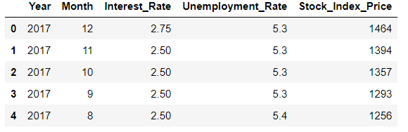 Data looks well imported
Identify variables that are interesting and scale them. Scale your data to be safe! You will not have a different outcome if you scale your data in spite of what anyone will tell you - this you can prove mathematically. My statement is true, as long as you do not consider floating-point stuff. If you have very large or very small numbers, then you have floating-point inaccuracy. And this can then lead to a lot of problems. And you get very large numbers and very small numbers by not scaling, to begin with. If you scale everything, to begin with, then everything looks the same. Everything is between minus two and plus two, everything is centered around zero. The reason why that is that most people will scale according will scale on use what is called a standard scaler, which is your normal or your Gaussian distribution. What you do is subtract away the mean, and then you divide by the standard deviation.
Another benefit to scaling is that if you use an iterative methodology, your data will generally converge faster if you have scaled it. But, as long as you have a linear system - there is a mathematical proof (this is a so-called convex problem) and if it is such, there is a specific solution in all cases, regardless of data scaling. In principle, you will not get more or less accuracy if you scale - however floating point inaccuracies are a thing to watch out for!
We keep "Interest_Rate" and "Unemployment_Rate" for further analysis:
text
x = df[['Interest_Rate','Unemployment_Rate']]
y = df['Stock_Index_Price']
text
# scale the data
from sklearn.preprocessing import StandardScaler
scaler = StandardScaler()
scaler.fit(x)
x = scaler.transform(x)
text
from sklearn.linear_model import LinearRegression
regression_model = LinearRegression()
# Fit the data(train the model)
regression_model.fit(x, y)
text
# predict
y_predicted = regression_model.predict(x)
text
print('Intercept: n', regression_model.intercept_) # pull out intercept
print('Coefficients: n', regression_model.coef_) # pull out coeffeicients
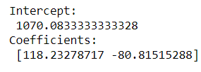 This output includes the intercept and coefficients to build the multiple linear regression equation.
N.B: We scaled the data, so the coefficients above reflect that. Nonetheless, there is a correlation between high-interest rates and stock prices rising and a smaller correlated effect with prices rising as unemployment falls. We can see that the scaled coefficients are roughly the same and are therefore directly comparable.
text
Stock_Index_Price = (Intercept) + (Interest_Rate coef)*X1 + (Unemployment_Rate coef)*X2
Plugging in new numbers:
text
Stock_Index_Price = (1070.083) + (118.233)*X1 + (-80.815)*X2
text
# prediction with sklearn
New_Interest_Rate = 2.75
New_Unemployment_Rate = 5.3
# create a scaled feature array and make the prediction
feature_array = scaler.transform([[New_Interest_Rate ,New_Unemployment_Rate]])
print ('Predicted Stock Index Price: n', regression_model.predict(feature_array))
 Given the new interest and unemployment rates, we expect the stock to be this price
Stats models
Same analysis but this time with sm. Again I stress the more important package to know is sklearn
text
# with statsmodels
X = sm.add_constant(x) # adding a constant

model = sm.OLS(y, X).fit()
predictions = model.predict(X)

print_model = model.summary()
print(print_model)
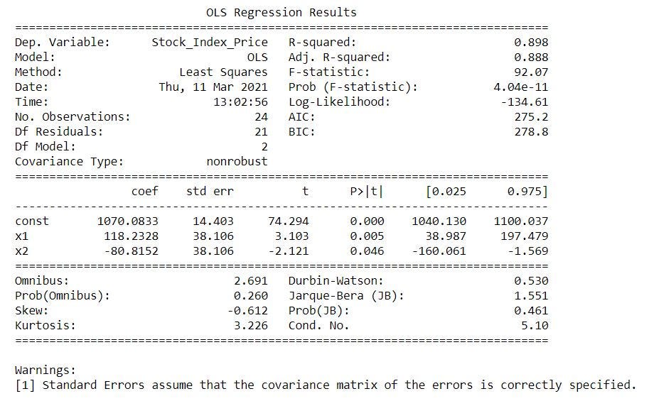 Adj R² is always lower than R² | We lose 2 degrees of freedom thanks to the multiple inputs
text
# Summary graphs:
import scipy.stats as stats
import statsmodels.api as statsmodels
from statsmodels.graphics.regressionplots import *
import seaborn as sns
import numpy as np
text
sns.distplot(model.resid, hist=True)
plt.grid(True)
plt.xlabel('Residual')
plt.ylabel('Frequency')
plt.title('Residual Histogram')
plt.show()
text
# Residuals vs Fitted Values
residuals = model.resid # outlier_linear = name of linear model on #our dataset
fitted_vals = model.predict(X) # making predictions from our fit #model
text
plt.plot(fitted_vals, residuals, 'o') # plotting predictions from #fit model vs residuals
text
plt.xlabel('Fitted Values')
plt.ylabel('Residuals')
plt.title('Residuals vs. Fitted Values (w/ 1 outlier)')
plt.show()
text
# create Q-Q plot to ensure normality
statsmodels.qqplot(residuals, stats.norm, fit=True, line='45')
text
# leverage Plot (Cook's Distance)
influence_plot(model) # from statsmodels.graphics.regressionplots #import *
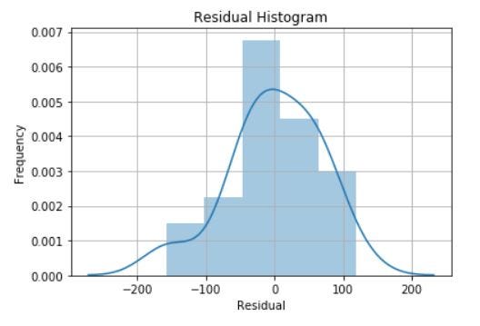 Residuals appear reasonably normally distributed
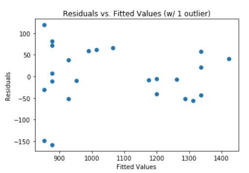 Residual plot, no apparent trend - residuals appear reasonably homoscedastic
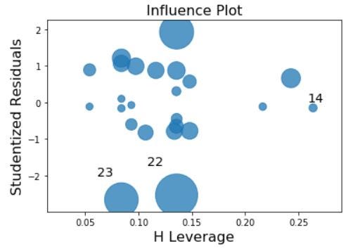 As expected, larger residual = larger influence on the fitted line | residuals are normalized (studentized)
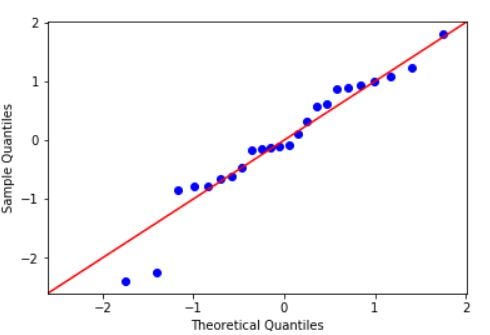 Data appears normally distributed, histogram confirmed
Conclusion
We have explored linear models in depth and run some Jupyter Notebook code cells to explore least-squares linear regression. Remember linear refers to the parameters - in the above stock example the data is multivariant: we used interest rates AND unemployment rates to predict a numeric outcome: the stock price GIVEN those inputs. The importance of homoscedasticity of the residuals was emphasized as was, albeit briefly, leverage and outliers.
In my next article, I will expand these concepts and explore using bootstrap with regression models!
Find me on Linkedin
Physicist cum Data Scientist- Available for new opportunity | SaaS | Sports | Start-ups | Scale-ups
Register Now to Continue Reading
Unlock Towards Data Science with a Free Account
All articles on Towards Data Science are available to registered users. Create a free account today to access this article and thousands more.
Register for freeSign in to your account
 Written By
See all from James Andrew Godwin
Data ScienceLinear Regression PythonMultiple LinearregressionTowards Data Science
Share This Article
Towards Data Science is a community publication. Submit your insights to reach our global audience and earn through the TDS Author Payment Program.
Write for TDS
Related Articles
Data Science
Following these rules has drastically improved my effectiveness as a data scientist to deliver more value from my work
Adam Sroka
June 27, 20229 min read
Artificial Intelligence
Full code examples on the MNIST dataset with VGG16 | ResNet50 | FG-UNET | Majority Voting | Single Transferable Vote | Instant-Runoff...
Cathie So, PhD
July 1, 20219 min read
Algorithms
How recasting propositional logic as sparse algebra leads to an elegant and efficient design
Dmitry Lesnik
October 30, 202516 min read
Data Science
Yelp data reveals cities with the most gun shops per capita
William Chon
December 26, 20203 min read
Machine Learning
Kmeans-Clustering, PCA
Benjamin Lau
January 8, 20197 min read
Artificial Intelligence
Helpful for your daily tasks
Pranjal Saxena
August 23, 20214 min read
Machine Learning
Make the most of Docker support in Lambda to host your models without the need for dedicated servers.
Jonathan Readshaw
June 20, 20213 min read
Artificial Intelligence
Powerful ways to use location analytics
Pranay Dave
February 22, 20225 min read
Programming
A beginner's guide to Python object comprehensions and protecting your home from a Joe Pesci-type burglar
Joe Marx
December 10, 20207 min read
Your home for data science and AI. The world's leading publication for data science, data analytics, data engineering, machine learning, and artificial intelligence professionals.
Subscribe to Our NewsletterWrite For TDS•About•Advertise•Privacy Policy•Terms of Use
© Insight Media Group, LLC 2026•The New Stack•roadmap.sh•Creator Network
Recommended Articles
Close