保留正文与补采附件。源页面当前未重新核验;具体限制见交付清单。
 We value your privacy
We use cookies to enhance your browsing experience, serve personalised ads or content, and analyse our traffic. By clicking "Accept All", you consent to our use of cookies.
Customise Reject All Accept All
Customise Consent Preferences
 We use cookies to help you navigate efficiently and perform certain functions. You will find detailed information about all cookies under each consent category below.
The cookies that are categorised as "Necessary" are stored on your browser as they are essential for enabling the basic functionalities of the site. ... Show more
NecessaryAlways Active
Necessary cookies are required to enable the basic features of this site, such as providing secure log-in or adjusting your consent preferences. These cookies do not store any personally identifiable data.
-
Cookie
BCTempID
-
Duration
10 minutes
-
Description
No description available.
-
Cookie
__cf_bm
-
Duration
1 hour
-
Description
This cookie, set by Cloudflare, is used to support Cloudflare Bot Management.
-
Cookie
AWSALBCORS
-
Duration
7 days
-
Description
Amazon Web Services set this cookie for load balancing.
-
Cookie
_cfuvid
-
Duration
session
-
Description
Cloudflare sets this cookie to track users across sessions to optimize user experience by maintaining session consistency and providing personalized services
-
Cookie
li_gc
-
Duration
6 months
-
Description
Linkedin set this cookie for storing visitor's consent regarding using cookies for non-essential purposes.
-
Cookie
__hssrc
-
Duration
session
-
Description
This cookie is set by Hubspot whenever it changes the session cookie. The __hssrc cookie set to 1 indicates that the user has restarted the browser, and if the cookie does not exist, it is assumed to be a new session.
-
Cookie
__hssc
-
Duration
1 hour
-
Description
HubSpot sets this cookie to keep track of sessions and to determine if HubSpot should increment the session number and timestamps in the __hstc cookie.
-
Cookie
wpEmojiSettingsSupports
-
Duration
session
-
Description
WordPress sets this cookie when a user interacts with emojis on a WordPress site. It helps determine if the user's browser can display emojis properly.
-
Cookie
BCSessionID
-
Duration
1 year 1 month 4 days
-
Description
Blueconic sets this cookie as a unique identifier for the BlueConic profile.
-
Cookie
_octo
-
Duration
1 year
-
Description
No description available.
-
Cookie
logged_in
-
Duration
1 year
-
Description
No description available.
-
Cookie
__Secure-YEC
-
Duration
past
-
Description
YouTube sets this cookie to stores the user's video player preferences using embedded YouTube video
-
Cookie
__eoi
-
Duration
6 months
-
Description
Description is currently not available.
-
Cookie
AWSALBTGCORS
-
Duration
7 days
-
Description
No description available.
-
Cookie
login-status-p
-
Duration
past
-
Description
Description is currently not available.
-
Cookie
AWSALBTG
-
Duration
7 days
-
Description
No description available.
-
Cookie
csrf_token
-
Duration
session
-
Description
No description available.
-
Cookie
token_v2
-
Duration
1 day
-
Description
Description is currently not available.
-
Cookie
D
-
Duration
1 year
-
Description
Description is currently not available.
-
Cookie
PHPSESSID
-
Duration
session
-
Description
This cookie is native to PHP applications. The cookie stores and identifies a user's unique session ID to manage user sessions on the website. The cookie is a session cookie and will be deleted when all the browser windows are closed.
-
Cookie
VISITOR_PRIVACY_METADATA
-
Duration
6 months
-
Description
YouTube sets this cookie to store the user's cookie consent state for the current domain.
-
Cookie
cookietest
-
Duration
session
-
Description
The cookietest cookie is typically used to determine whether the user's browser accepts cookies, essential for website functionality and user experience.
-
Cookie
__Host-airtable-session
-
Duration
1 year
-
Description
This cookie is used to enable us to integrate the services of Airtable.
-
Cookie
__Host-airtable-session.sig
-
Duration
1 year
-
Description
This cookie is used to enable us to integrate the services of Airtable.
-
Cookie
m
-
Duration
1 year 1 month 4 days
-
Description
Stripe sets this cookie for fraud prevention purposes. It identifies the device used to access the website, allowing the website to be formatted accordingly.
-
Cookie
BIGipServer*
-
Duration
session
-
Description
Marketo sets this cookie to collect information about the user's online activity and build a profile about their interests to provide advertisements relevant to the user.
-
Cookie
__cfruid
-
Duration
session
-
Description
Cloudflare sets this cookie to identify trusted web traffic.
-
Cookie
_GRECAPTCHA
-
Duration
6 months
-
Description
Google Recaptcha service sets this cookie to identify bots to protect the website against malicious spam attacks.
-
Cookie
__Secure-YNID
-
Duration
6 months
-
Description
Google cookie used to protect user security and prevent fraud, especially during the login process.
-
Cookie
cookieyes-consent
-
Duration
1 year
-
Description
CookieYes sets this cookie to remember users' consent preferences so that their preferences are respected on subsequent visits to this site. It does not collect or store any personal information about the site visitors.
Functional
Functional cookies help perform certain functionalities like sharing the content of the website on social media platforms, collecting feedback, and other third-party features.
-
Cookie
lidc
-
Duration
1 day
-
Description
LinkedIn sets the lidc cookie to facilitate data center selection.
-
Cookie
brw
-
Duration
1 year
-
Description
No description available.
-
Cookie
brwConsent
-
Duration
5 minutes
-
Description
Description is currently not available.
-
Cookie
WMF-Uniq
-
Duration
1 year
-
Description
Description is currently not available.
-
Cookie
loom_anon_comment
-
Duration
1 year
-
Description
No description available.
-
Cookie
loom_referral_video
-
Duration
session
-
Description
Description is currently not available.
-
Cookie
VISITOR_INFO1_LIVE
-
Duration
6 months
-
Description
A cookie set by YouTube to measure bandwidth that determines whether the user gets the new or old player interface.
-
Cookie
yt-remote-connected-devices
-
Duration
Never Expires
-
Description
YouTube sets this cookie to store the user's video preferences using embedded YouTube videos.
-
Cookie
ytidb::LAST_RESULT_ENTRY_KEY
-
Duration
Never Expires
-
Description
The cookie ytidb::LAST_RESULT_ENTRY_KEY is used by YouTube to store the last search result entry that was clicked by the user. This information is used to improve the user experience by providing more relevant search results in the future.
-
Cookie
yt-remote-device-id
-
Duration
Never Expires
-
Description
YouTube sets this cookie to store the user's video preferences using embedded YouTube videos.
-
Cookie
yt-remote-session-name
-
Duration
session
-
Description
The yt-remote-session-name cookie is used by YouTube to store the user's video player preferences using embedded YouTube video.
-
Cookie
yt-remote-fast-check-period
-
Duration
session
-
Description
The yt-remote-fast-check-period cookie is used by YouTube to store the user's video player preferences for embedded YouTube videos.
-
Cookie
yt-remote-session-app
-
Duration
session
-
Description
The yt-remote-session-app cookie is used by YouTube to store user preferences and information about the interface of the embedded YouTube video player.
-
Cookie
yt-remote-cast-available
-
Duration
session
-
Description
The yt-remote-cast-available cookie is used to store the user's preferences regarding whether casting is available on their YouTube video player.
-
Cookie
yt-remote-cast-installed
-
Duration
session
-
Description
The yt-remote-cast-installed cookie is used to store the user's video player preferences using embedded YouTube video.
-
Cookie
cp_session
-
Duration
3 months
-
Description
Codepen sets this cookie for Help systems found in the website.
-
Cookie
loid
-
Duration
1 year 1 month 4 days
-
Description
This cookie is set by the Reddit. The cookie enables the sharing of content from the website onto the social media platform.
Analytics
Analytical cookies are used to understand how visitors interact with the website. These cookies help provide information on metrics such as the number of visitors, bounce rate, traffic source, etc.
-
Cookie
__hstc
-
Duration
6 months
-
Description
Hubspot set this main cookie for tracking visitors. It contains the domain, initial timestamp (first visit), last timestamp (last visit), current timestamp (this visit), and session number (increments for each subsequent session).
-
Cookie
hubspotutk
-
Duration
6 months
-
Description
HubSpot sets this cookie to keep track of the visitors to the website. This cookie is passed to HubSpot on form submission and used when deduplicating contacts.
-
Cookie
_ga
-
Duration
1 year 1 month 4 days
-
Description
Google Analytics sets this cookie to calculate visitor, session and campaign data and track site usage for the site's analytics report. The cookie stores information anonymously and assigns a randomly generated number to recognise unique visitors.
-
Cookie
ga*
-
Duration
1 year 1 month 4 days
-
Description
Google Analytics sets this cookie to store and count page views.
-
Cookie
__Host-psifi.analyticsTrace
-
Duration
6 hours
-
Description
Description is currently not available.
-
Cookie
__Host-psifi.analyticsTraceV2
-
Duration
6 hours
-
Description
Description is currently not available.
-
Cookie
_gh_sess
-
Duration
session
-
Description
GitHub sets this cookie for temporary application and framework state between pages like what step the user is on in a multiple step form.
-
Cookie
YSC
-
Duration
session
-
Description
YSC cookie is set by Youtube and is used to track the views of embedded videos on Youtube pages.
-
Cookie
ajs_anonymous_id
-
Duration
1 year
-
Description
This cookie is set by Segment to count the number of people who visit a certain site by tracking if they have visited before.
-
Cookie
vuid
-
Duration
1 year 1 month 4 days
-
Description
Vimeo installs this cookie to collect tracking information by setting a unique ID to embed videos on the website.
Performance
Performance cookies are used to understand and analyse the key performance indexes of the website which helps in delivering a better user experience for the visitors.
-
Cookie
AWSALB
-
Duration
7 days
-
Description
AWSALB is an application load balancer cookie set by Amazon Web Services to map the session to the target.
-
Cookie
acq
-
Duration
past
-
Description
Description is currently not available.
-
Cookie
acq.sig
-
Duration
past
-
Description
Description is currently not available.
-
Cookie
ptc
-
Duration
2 years
-
Description
No description available.
Advertisement
Advertisement cookies are used to provide visitors with customised advertisements based on the pages you visited previously and to analyse the effectiveness of the ad campaigns.
-
Cookie
muc_ads
-
Duration
1 year 1 month 4 days
-
Description
Twitter sets this cookie to collect user behaviour and interaction data to optimize the website.
-
Cookie
guest_id_marketing
-
Duration
1 year 1 month 4 days
-
Description
Twitter sets this cookie to identify and track the website visitor.
-
Cookie
guest_id_ads
-
Duration
1 year 1 month 4 days
-
Description
Twitter sets this cookie to identify and track the website visitor.
-
Cookie
personalization_id
-
Duration
1 year 1 month 4 days
-
Description
Twitter sets this cookie to integrate and share features for social media and also store information about how the user uses the website, for tracking and targeting.
-
Cookie
guest_id
-
Duration
1 year 1 month 4 days
-
Description
Twitter sets this cookie to identify and track the website visitor. It registers if a user is signed in to the Twitter platform and collects information about ad preferences.
-
Cookie
bcookie
-
Duration
1 year
-
Description
LinkedIn sets this cookie from LinkedIn share buttons and ad tags to recognize browser IDs.
-
Cookie
__Secure-ROLLOUT_TOKEN
-
Duration
6 months
-
Description
YouTube sets this cookie to manage feature rollout and experimentation. It helps Google control which new features or interface changes are shown to users as part of testing and staged rollouts, ensuring consistent experience for a given user during an experiment.
-
Cookie
yt.innertube::nextId
-
Duration
Never Expires
-
Description
YouTube sets this cookie to register a unique ID to store data on what videos from YouTube the user has seen.
-
Cookie
yt.innertube::requests
-
Duration
Never Expires
-
Description
YouTube sets this cookie to register a unique ID to store data on what videos from YouTube the user has seen.
-
Cookie
session_tracker
-
Duration
session
-
Description
This cookie is set by the Reddit. This cookie is used to identify trusted web traffic. It also helps in adverstising on the website.
-
Cookie
edgebucket
-
Duration
session
-
Description
Reddit sets this cookie to save the information about a log-on Reddit user, for the purpose of advertisement recommendations and updating the content.
-
Cookie
did
-
Duration
1 year
-
Description
Arbor sets this cookie to show targeted ads to site visitors.This cookie expires after 2 months or 1 year.
Uncategorised
Other uncategorised cookies are those that are being analysed and have not been classified into a category as yet.
No cookies to display.
Reject All Save My Preferences Accept All
Toggle SearchToggle Mobile Navigation
Publish AI, ML & data-science insights to a global community of data professionals.
Sign inSubmit an Article
LatestEditor's PicksNewsletterShipAI
Write For TDS
LinkedInXToggle Search
Artificial Intelligence
Monitoring Machine Learning Models in Production: Why and How?
How our model is impacted in the evolving world? An analysis focusing on drift examples, and implementing Python-based monitoring...
John Leung
September 5, 202312 min read
How is our model impacted in the evolving world? An analysis focusing on drift examples, and implementing Python-based monitoring strategies
Machine Learning (ML) model development often takes time and requires technical expertise. As data science enthusiasts, when we acquire a dataset to explore and analyze, we eagerly train and validate it using diverse state-of-the-art models or employing data-centric strategies. It feels incredibly fulfilling when we optimize the model's performance as if all the tasks have been accomplished.
However, after deploying the model to production, there are plenty of reasons that contribute to lower model performance or degradation.
 Photo by Adrien Delforge on Unsplash
#1 The training data is generated through simulation
Learn this step by step with the interactive AI Engineer, Data Analyst and Machine Learning roadmaps.
Data scientists often face limitations in accessing the production data, which results in training the model using simulated or sample data instead. While data engineers bear the responsibility of ensuring the representativeness of the training data in terms of scale and complexity, the training data still deviates to some extent from the production data. There is also a risk of systematic flaws in upstream data processing, such as data collection and labeling. These factors can impact the extraction of additional useful input features or hinder the model's ability to generalize well.
Example: Investor data in the financial industry or patient information in the healthcare industry is often simulated due to security and privacy concerns.
#2 The new production data exhibits a new data distribution
Over time, the characteristics of input features can also change, such as shifts in age groups, income ranges, or other customer demographics. The data source itself may even be completely replaced due to various cases. During the model development process, optimization relies on learning and capturing patterns from the majority group within the training data. However, as time progresses, the previous majority may transition into the minority in the production data, rendering the original static model inadequate for meeting the most recent production needs.
Example: The model is well trained initially using customer data in Asian regions. Recently since the business expands into the United States, the same model directly makes prediction based on the input features which have exhibited variations.
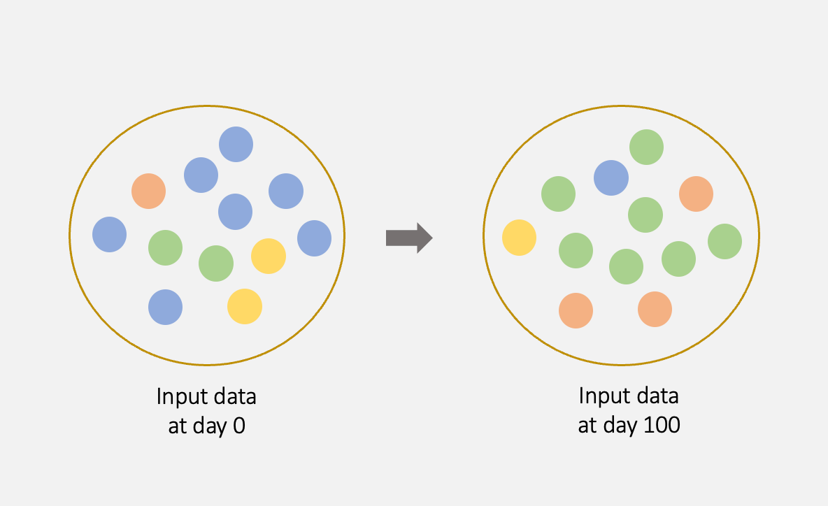 Data drift (Image by author)
#3 The patterns that we predict are evolving
Apart from shifts in the distribution of input features, the relationship between the features and the target variable can also change in the evolving environment. These changes can occur in unexpected ways over time, rendering the original model progressively ineffective.
These changes can occur abruptly, sometimes within a few weeks, due to unforeseen circumstances.
Example: The surge in demand for virtual meeting services during public COVID-19 lockdowns.
This type of change takes longer to manifest and is often a natural progression.
Example: The gradual increase in the price of dairy products due to long-term inflation.
These changes can happen periodically, often during specific times of the year.
Example: The rapid growth in e-commerce sales during various special days like Black Friday and the Saturday before Christmas.
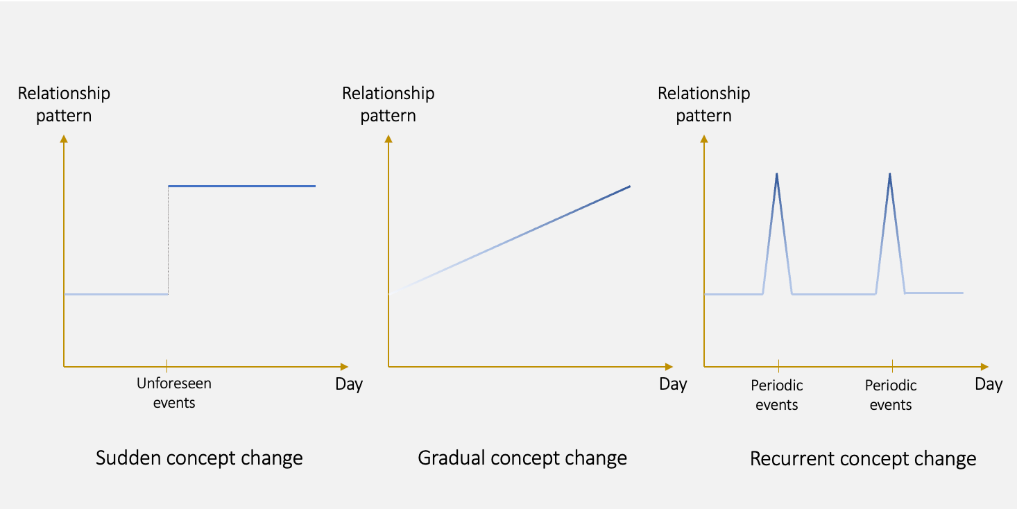 Concept drift (Image by author)
Model development is only a tiny part of a production-ready ML system
Many companies emphasize data-driven decision-making through the use of ML applications. Imagine that your ML models are utilized in critical applications, such as medical diagnosis, to support healthcare professionals in identifying diseases and conditions. Any model degradation means impacting the accuracy of diagnoses, potentially resulting in incorrect treatment plans and compromised patient outcomes. There are tons of cases with high importance in the real world, thus it becomes imperative to implement objective and continuous monitoring to detect any possible shifts.
In the following sections, we will delve into various layers of monitoring and provide illustrative Python code examples to demonstrate their implementation.
 Photo by Nathy dog on Unsplash
1 Monitor the model performance metrics
To detect any sign of model degradation, one of the direct and effective ways is to keep track of the performance metrics over time.
These performance metrics collected from the initial deployment serve as benchmarks for ongoing monitoring and evaluation. Periodically reassessing them is crucial whenever a new batch of ground truth data is collected, such as upon completion of a marketing campaign. If the error metrics rise above a predefined threshold, or if the metrics such as R-squared fall below the threshold, it is necessary to consider re-executing the data engineering process and retraining the model.
While this monitoring approach provides valuable insights into any drifts, it tends to lag. We can take a more proactive approach to monitor the latest input data.
2 Detect the changes in data distribution
Instead of waiting for sufficient input data for reliable evaluation of model performance, we can apply statistical methods for comparing the data distributions of two datasets. In our case, we can determine if the distribution of the training dataset is the same as that of the latest production dataset. If it is not statistically confident that two distributions are the same, it suggests a drift in the model. This is as a proxy for performance changes.
- Kolmogorov-Smirnov Test (K-S Test): nonparametric test (i.e. with no assumption on the underlying data distribution) for numeric features , it is more sensitive near the center of the distribution than at the tails.
Interpretation: When p-value < 0.05, an alert indicating the presence of a drift is triggered.
- Population Stability Index (PSI): A statistical test that can be applied to both numeric and categorical variables. It is a metric that shows how each variable has diverged independently from the baseline values. It is sometimes called the Characteristic Stability Index (CSI) when evaluating the distribution of features rather than target variables.
Interpretation: A value 0~0.1 means no significant distribution change; a value 0.1~0.2 considered a moderate distribution change; and a value larger than 0.2 interpreted as a significant distribution change.
Other famous statistical tests include Kullback-Leibler divergence, Jensen-Shannon divergence, and Wasserstein distance.
3 Monitor drift using a sliding window approach
Any delay in detecting data or pattern drifts results in a time gap, potentially leading to discrepancies between the ground truth and model predictions. To bridge the gap, are there any further advancements available? One promising idea is leveraging streaming data instead of batch data.
The Adaptive Windowing (ADWIN) algorithm utilizes a sliding window approach to effectively detect concept drift. Unlike traditional fixed-size windows, ADWIN decides the size of the window by cutting the statistics window at different points. Whenever newly arriving data comes, ADWIN analyses the statistics and identifies the point at which two sub-windows demonstrate notable differences in their means.
Interpretation: When the absolute difference between the two means exceeds a pre-defined threshold, an alert indicating the presence of a drift is triggered.
Example Walkthrough
Let's explore an example that demonstrates the implementation of the above monitoring strategies.
We will utilize a dataset obtained from Kaggle. The dataset comprises 100k records, encompassing 28 features **** that describe the customer demographics and their credit-related history.
Our objective is to segregate customers in a global financial company into credit score brackets. The target variable is Credit_Score , a categorical measure classified as 'Poor', 'Standard', and 'Good'.
Examples of features include:
- Occupation : Occupation of the customers (e.g. scientist, teacher, engineer, etc.)
- _Annual Income : Annual income of the customers
- _Credit_History Age : The age of customers' credit history
- _Payment Behaviour : 6 groups of payment behaviors based on spending frequency (low/ high) and payment amount (small/ medium/ large)
 Photo by CardMapr.nl on Unsplash
Model performance metrics
Let's start by applying data cleansing and transformation techniques, including but not limited to:
- Correcting/ Removing records with missing values or incorrect data (e.g. age < 0), or duplicates
- Detecting and handling data outliers
- Performing min-max scaling on numeric variables
- Applying label encoding on categorical variables
This part requires in-depth exploratory data analysis. However, since the focus is on sharing the monitoring strategies, the transformations performed are not discussed in detail here.
Afterward, we split the dataset and developed the advanced gradient boosting algorithm, LightGBM.
python
import numpy as np
import pandas as pd
from sklearn import metrics
from sklearn.metrics import f1_score, precision_score, recall_score
from sklearn.model_selection import train_test_split
from sklearn.preprocessing import LabelEncoder
from lightgbm import LGBMClassifier

# Convert target variable to numeric
df['Credit_Score'] = df['Credit_Score'].str.replace('Good', '3', n=-1)
df['Credit_Score'] = df['Credit_Score'].str.replace('Standard', '2', n=-1)
df['Credit_Score'] = df['Credit_Score'].str.replace('Poor', '1', n=-1)
df['Credit_Score'] = df[['Credit_Score']].apply(pd.to_numeric)

# Split the dataset
X=df.loc[:, df.columns != 'Credit_Score']
Y=df['Credit_Score']
x_train, x_test, y_train, y_test = train_test_split(X, Y, test_size=0.25)

# Train the LightGBM model
lgbm = LGBMClassifier()
lgbm.fit(x_train, y_train)
y_pred = lgbm.predict(x_test)

# Print performance metrics
print('F1 score: %.3f' % f1_score(y_test, y_pred, average='weighted'))
print('Precision: %.3f' % precision_score(y_test, y_pred, average='weighted'))
print('Recall: %.3f' % recall_score(y_test, y_pred, average='weighted'))
During our model development, we gathered several performance metrics, including an F1 score of 0.810, a precision score of 0.818, and a recall score of 0.807. Subsequent monitoring can be evaluated similarly. For instance, if the F1 score falls below 0.75, it serves as an alert, prompting us to take immediate action to mitigate the issue.
K-S Test
To demonstrate how the K-S Test works, I have selected a numeric feature _Credit_History Age. We will examine the sensitivity of this statistical test by creating three distinct datasets: one with 1000 samples, another with 5000 samples, and a third with approximately 64000 samples, which corresponds to the total size of the cleaned training samples. Each data point within the _Credit_History Age feature has been randomly picked from the training data and altered by a random floating-point number.
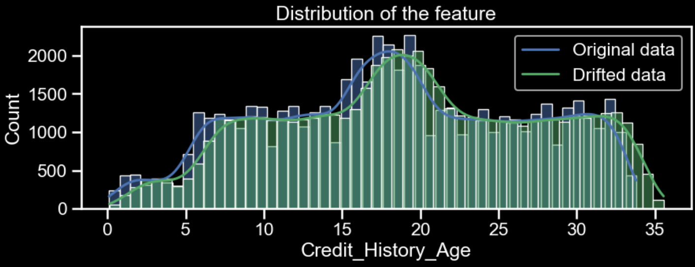 Data distributions of 'Credit_History_Age' in original data and drifted data (Image by author)
We obtained the following results:
- For the dataset with 1000 samples, the p-value of the K-S Test is 0.093.
- For the dataset with 5000 samples, the p-value of the K-S Test is 0.002.
- For the dataset with around 64000 samples, the p-value of the K-S Test is 0.000.
When examining the data drift scenario using 1000 samples, the p-value exceeded 0.05. Consequently, we can conclude that the two distributions remain similar. However, as the sample size increased to 5000 and beyond, the K-S Test exhibited exceptional performance, yielding p-values significantly lower than 0.05. This provides a clear indication of a data distribution drift, serving as a clear alert.
python
from scipy import stats

# Create new datasets with different no. of samples
original_df = x_train[['Credit_History_Age', 'Payment_Behaviour']].reset_index(drop=True)
new_df = x_train[['Credit_History_Age', 'Payment_Behaviour']].reset_index(drop=True)
new_df1 = new_df.sample(n = 1000).reset_index(drop=True)
new_df2 = new_df.sample(n = 5000).reset_index(drop=True)
new_df3 = new_df.sample(n = len(x_train)).reset_index(drop=True)

# Prepare drifted data for numeric feature
def drift_numeric_col(df, numeric_col, drift_range):
    df[numeric_col] = df[numeric_col] + np.random.uniform(0, drift_range, size=(df.shape[0], ))

drift_numeric_col(new_df1, 'Credit_History_Age', 2)
drift_numeric_col(new_df2, 'Credit_History_Age', 2)
drift_numeric_col(new_df3, 'Credit_History_Age', 2)

# K-S Test
def ks_test(original_df, new_df, numeric_col):
    test = stats.ks_2samp(original_df[numeric_col], new_df[numeric_col])
    print("Column : %s , p-value : %1.3f" % (numeric_col, test[1]))

# Conduct K-S Test for numeric feature
ks_test(original_df, new_df1, 'Credit_History_Age')
ks_test(original_df, new_df2, 'Credit_History_Age')
ks_test(original_df, new_df3, 'Credit_History_Age')
PSI
In addition to utilizing the K-S Test, we will also leverage the PSI (Population Stability Index) to evaluate the numeric feature _Credit_History Age and assess the categorical feature _Payment Behaviour. To represent the drift effect, we have randomly replaced 80% of the data of the feature _Payment Behaviour with specific label values.
python
# Prepare drifted data for categorical column
def drift_cat_col(df, cat_col, drift_ratio):
    no_of_drift = round(len(df)*drift_ratio)
    random_numbers = [random.randint(0, 1) for _ in range(no_of_drift)]
    indices = random.sample(range(len(df[cat_col])), no_of_drift)
    df.loc[indices, cat_col] = random_numbers

drift_cat_col(new_df1, 'Payment_Behaviour', 0.8)
drift_cat_col(new_df2, 'Payment_Behaviour', 0.8)
drift_cat_col(new_df3, 'Payment_Behaviour', 0.8)
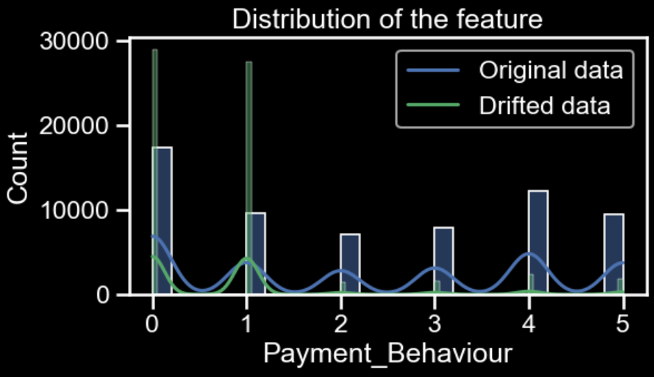 Data distributions of 'Payment_Behaviour' in original data and drifted data (Image by author)
- Numeric feature _Credit_History Age
With a sample size of 1000, the PSI value is 0.023.
With a sample size of 5000, the PSI value is 0.015.
With a sample size of approximately 64000, the PSI value is 0.021.
- Categorical feature _Payment Behaviour
With a sample size of 1000, the PSI value is 0.108.
With a sample size of 5000, the PSI value is 0.111.
With a sample size of approximately 64000, the PSI value is 0.112.
All the PSI values for the _Credit_History Age feature are significantly lower than 0.1, indicating no significant distribution change. By comparing these results with those obtained from the K-S Test, we observe that the K-S Test exhibits greater sensitivity in detecting distribution changes compared to PSI.
On the other hand, the PSI values for the _Payment Behaviour feature are around 0.11, signifying a moderate distribution change. Interestingly, the three PSI values remain relatively consistent, implying that PSI's effectiveness is less dependent on sample sizes. Besides, PSI has the flexibility to monitor across various feature types, positioning it still a valuable approach for drift detection.
Below is the implementation code of PSI:
python
def psi(data_base, data_new, num_bins = 10):
    # Sort the data
    data_base = sorted(data_base)
    data_new = sorted(data_new)

    # Prepare the bins
    min_val = min(data_base[0], data_new[0])
    max_val = max(data_base[-1], data_new[-1])
    bins = [min_val + (max_val - min_val)*(i)/num_bins for i in range(num_bins+1)]
    bins[0] = min_val - 0.0001
    bins[-1] = max_val + 0.0001

    # Bucketize the baseline data and count the samples
    bins_base = pd.cut(data_base, bins = bins, labels = range(1,num_bins+1))
    df_base = pd.DataFrame({'base': data_base, 'bin': bins_base})
    grp_base = df_base.groupby('bin').count()
    grp_base['percent_base'] = grp_base['base'] / grp_base['base'].sum()

    # Bucketize the new data and count the samples
    bins_new = pd.cut(data_new, bins = bins, labels = range(1,num_bins+1))
    df_new = pd.DataFrame({'new': data_new, 'bin': bins_new})
    grp_new = df_new.groupby('bin').count()
    grp_new['percent_new'] = grp_new['new'] / grp_new['new'].sum()

    # Compare the bins
    psi_df = grp_base.join(grp_new, on = "bin", how = "inner")

    # Calculate the PSI
    psi_df['percent_base'] = psi_df['percent_base'].replace(0, 0.0001)
    psi_df['percent_new'] = psi_df['percent_new'].replace(0, 0.0001)
    psi_df['psi'] = (psi_df['percent_base'] - psi_df['percent_new']) * np.log(psi_df['percent_base'] / psi_df['percent_new'])

    # Return the total PSI value
    return np.sum(psi_df['psi'].values)

# Conduct K-S Test for numeric feature
psi(original_df['Credit_History_Age'], new_df1['Credit_History_Age'])
psi(original_df['Credit_History_Age'], new_df2['Credit_History_Age'])
psi(original_df['Credit_History_Age'], new_df3['Credit_History_Age'])

# Conduct K-S Test for categorical feature
psi(original_df['Payment_Behaviour'], new_df1['Payment_Behaviour'])
psi(original_df['Payment_Behaviour'], new_df2['Payment_Behaviour'])
psi(original_df['Payment_Behaviour'], new_df3['Payment_Behaviour'])
ADWIN algorithm
Lastly, we test the power of ADWIN in detecting the change in the numeric feature _Credit_History Age. The data stream consists of the training data, followed by the drifted data. We expect that the algorithm will promptly identify the drift shortly after examining the entirety of the original data.
To visually represent the situation, a scatter plot is created to showcase the final 500 points of the original data in blue, followed by the initial 500 points of the drifted data, depicted in green. The drifted data exhibits a slightly higher average value.
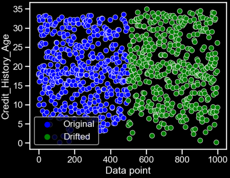 Scatter plot (Image by author)
By continuously adding stream elements, ADWIN identifies the change at index 64457, which is the 637th data point within the drifted data. In comparison, the K-S Test and PSI necessitate a larger number of data points to conclude the presence of a drift confidently. The better performance of ADWIN is a testament to its capability to monitor diverse features at speed and ease.
Below is the implementation code of ADWIN:
python
from skmultiflow.drift_detection import ADWIN

adwin = ADWIN()
data_stream=[]
data_stream = np.concatenate((original_df['Credit_History_Age'],new_df3['Credit_History_Age']))

# Add stream elements to ADWIN and verify if drift occurred
for i in range(len(data_stream)):
  adwin.add_element(data_stream[i])
  if adwin.detected_change():
  print('Change detected at index {}'.format(i))
  adwin.reset()
Wrapping it up
We've delved into the crucial concepts of data drift and model drift, which can lead to model decay in production. We can proactively monitor and detect drift conditions using model performance metrics, statistical tests, and adaptive windowing techniques. Unlike participating in a one-time Kaggle competition, building a production-ready ML system is an iterative journey. It requires a mindset shift towards integrating comprehensive model monitoring to ensure a robust and consistently high-performance serving space.
Before you go
If you enjoy this reading, I invite you to **** follow my Medium page. By doing so, you can stay updated with exciting content related to data science side projects, Machine Learning Operations (MLOps) demonstrations, and project management methodologies.
Optimizing Your Strategies with Approaches Beyond A/B Testing
How to Apply Data-centric AI Mindset to Text Classification Problems?
Register Now to Continue Reading
Unlock Towards Data Science with a Free Account
All articles on Towards Data Science are available to registered users. Create a free account today to access this article and thousands more.
Register for freeSign in to your account
 Written By
See all from John Leung
Artificial IntelligenceMachine LearningMlopsPythonStatistics
Share This Article
Towards Data Science is a community publication. Submit your insights to reach our global audience and earn through the TDS Author Payment Program.
Write for TDS
Related Articles
Programming
An example of extracting text with keywords with Regular Expression.
KahEm Chu
April 10, 20215 min read
Artificial Intelligence
Surprise, surprise. It's not as hard as I thought it would be.
Arunn Thevapalan
March 16, 202414 min read
Data Science
The article discusses memoization using the Python standard library. The functools.lru_cache decorator makes this so simple!
Marcin Kozak
November 11, 202312 min read
Artificial Intelligence
Every Monday, I present 4 publications from my research area. Let's discuss them! [← Previous...
Quentin Gallouédec
May 17, 20215 min read
Machine Learning
The bedrock utility helps keep code modular and levels up your iteration speed
Sean Easter
March 1, 202211 min read
Artificial Intelligence
Understanding the importance of monitoring the ML and deep learning models after production can have a significant impact that these models...
Suhas Maddali
June 28, 20226 min read
Machine Learning
Using Python to automate the process of setting up new project directories and making the first commit to a new repository in Github
Jack Leitch
December 21, 20204 min read
Machine Learning
As someone who has overseen and created thousands of machine learning models, I want to share some of the most important insights learned.
Dr. Xuxu Wang
July 21, 20205 min read
Machine Learning
Classifying edible and poisonous mushrooms with CatBoost gradient boosted decision trees
Caroline Arnold
August 17, 20235 min read
Your home for data science and AI. The world's leading publication for data science, data analytics, data engineering, machine learning, and artificial intelligence professionals.
Subscribe to Our NewsletterWrite For TDS•About•Advertise•Privacy Policy•Terms of Use
© Insight Media Group, LLC 2026•The New Stack•roadmap.sh•Creator Network
Recommended Articles
Close