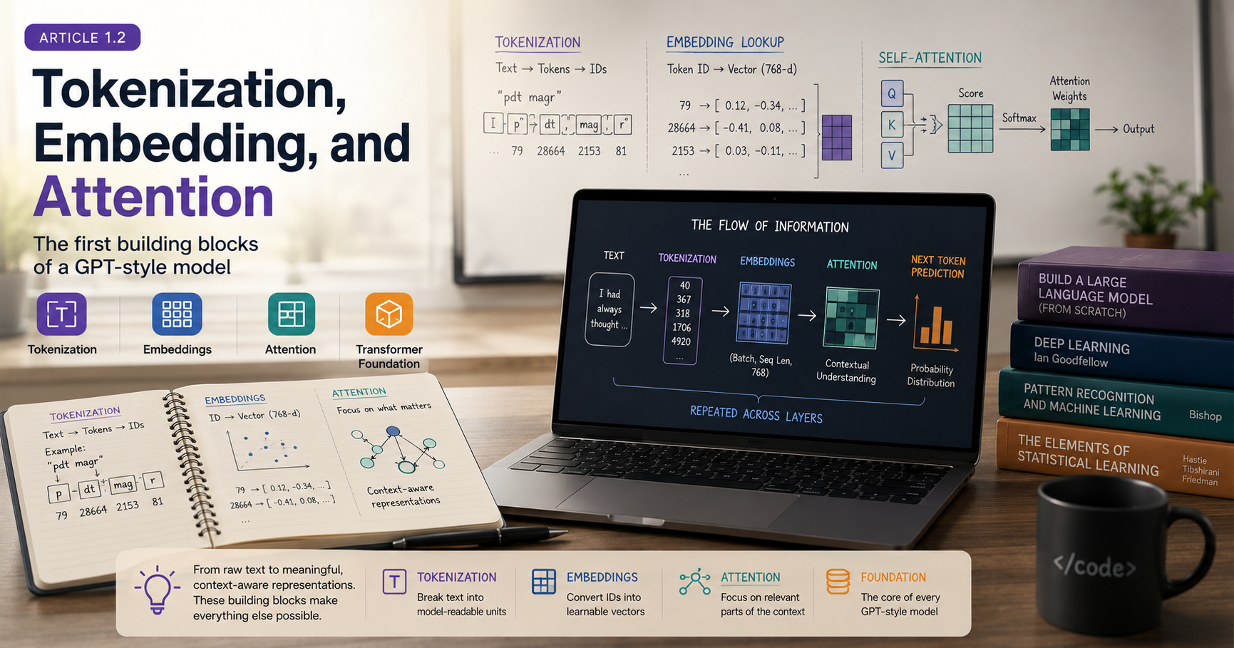
How raw text becomes token IDs, embeddings, and context-aware representations inside a GPT-2-style model.
In the first article, I shared why I decided to build a GPT-style model from scratch and what I ultimately built. In this article, I want to open that box and look at the first set of building blocks that make the model work:
Tokenization
Preparing the training data
Embeddings
The attention mechanism
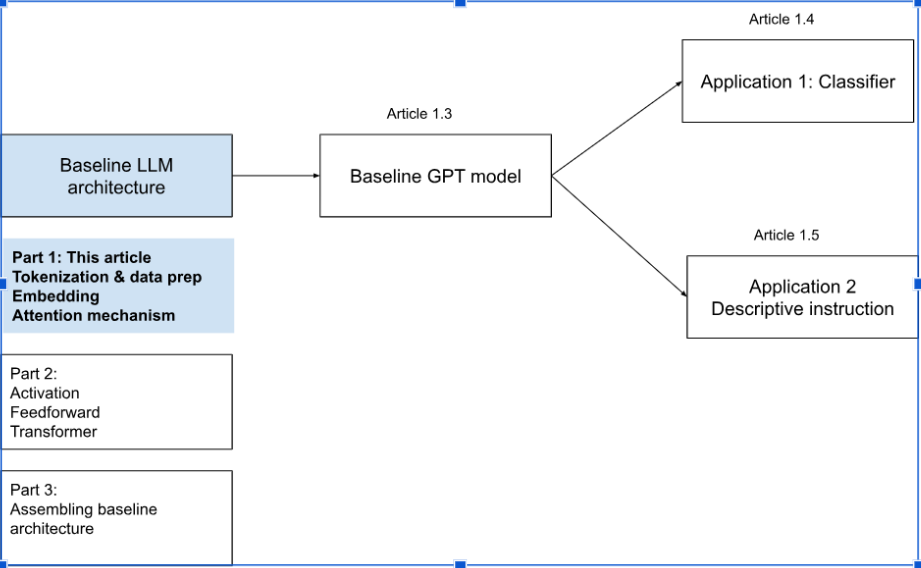
This is not intended to be an exhaustive technical walkthrough. There is far more happening in the code than I can reasonably cover in one article. Instead, I will focus on the key ideas and configurations that appear in the accompanying GitHub repository and explain how they shape the model.
To help us keep track, I will use the following GPT-2 Small-style configuration throughout the article:
GPT_CONFIG_124M = {
    "vocab_size": 50_257,
    "context_length": 1_024,
    "emb_dim": 768,
    "n_heads": 12,
    "n_layers": 12,
    "drop_rate": 0.1,
    "qkv_bias": False,
}
I will also keep calling out the dimensions of the tensors as they move through the model. Personally, I found dimensions to be one of the easiest ways to understand what the code was actually doing.
Before an LLM can train on text, the text must be converted into tokens and then into token IDs.
A tokenizer has a finite vocabulary: the complete set of tokens it knows. In our configuration, vocab_size = 50,257, which means every token produced by the tokenizer must map to one of 50,257 token IDs.
This does not mean that the vocabulary contains every possible English word. GPT-2 uses Byte Pair Encoding, or BPE, which can split unfamiliar text into smaller units that already exist in the vocabulary.
For example, some random text such as:
pdt magr
may be split into:
Tokens:    ['p', 'dt', ' mag', 'r']
Token IDs: [79, 28664, 2153, 81]
The model never directly receives the original string. It receives the sequence of token IDs.
Tokenization is also sensitive to the exact text. Capitalization, pluralization, and even a preceding space can change the result:
'cat'  → ['cat']     → [9246]
'Cat'  → ['Cat']     → [21979]
'CAT'  → ['C', 'AT'] → [34, 1404]
'cats' → ['cats']    → [24619]
This was one of my first useful realizations: a word is not necessarily a token, and the same-looking word can be represented differently depending on how it appears in the text.
Once the text has been converted into token IDs, the next step is to create examples the model can learn from.
The basic training objective is simple: given the tokens so far, predict the next token.
Suppose our tokenized text is conceptually:
[I, had, always, thought, Jack, Gisburn, is, my, friend]
Let us define a basic strategy with:
context_length = 5: Each training example contains five input tokens.
The target sequence, or output, is created by shifting the input tokens one position to the right while keeping both sequences the same length. During training, the model predicts the next token at every position in the sequence. During generation, however, we usually use only the prediction from the final position to select the next token.
stride = 2: The next example begins two positions after the previous one. The stride determines how much consecutive training samples overlap. A smaller stride creates more examples and uses the text more thoroughly, but it also creates more redundancy. A larger stride reduces overlap but may skip some possible training windows.
The first input-target pair would be:
Input 1:  [I, had, always, thought, Jack]
Target 1: [had, always, thought, Jack, Gisburn]
The target is simply the input sequence shifted one position to the right.
With a stride of two, the next pair becomes:
Input 2:  [always, thought, Jack, Gisburn, is]
Target 2: [thought, Jack, Gisburn, is, my]
During pretraining, the model makes a next-token prediction at every position. For the first example, it learns to predict:
I       → had
had     → always
always  → thought
thought → Jack
Jack    → Gisburn
This data-preparation strategy also changes with the use case. For language-model pretraining, the target is the next-token sequence. For classification fine-tuning, the target may instead be a class such as spam or not spam. The model architecture may remain largely familiar, but the way we construct the input and output data changes substantially.
In the GitHub repository, the dataset and data-loader classes handle this preparation and convert the raw text into batches that the model can process.
At this point, our input consists of token IDs. These numbers are only identifiers.
For example, token ID 9246 does not carry any mathematical meaning by itself. It does not tell the model that cat is an animal, that it may be a pet, or that it is related to dog. It simply identifies one row in the vocabulary.
To build intuition, imagine a toy embedding space with only three dimensions:
Dimension 1: association with pets
Dimension 2: association with wildlife
Dimension 3: association with sports
Tokens might appear at hypothetical locations such as:
cat     → [2.0, 0.1, 0.0]
horse   → [1.2, 0.8, 2.0]
cricket → [0.2, 4.0, 8.0]
In this simplified example, horse has associations with pets, wildlife, and sports, while cricket may be associated with both an animal and a sport.
Real embeddings do not come with dimensions labelled pet, wildlife, or sport. The individual dimensions have no predefined meanings. The model learns a distributed representation across hundreds of dimensions, and understanding what these internal representations capture is itself an active field of research.
The embedding values also do not start with meaningful coordinates. They begin as random numbers and are adjusted during training. When tokens repeatedly appear in similar contexts, the model may learn representations that place them closer together or make them useful in similar computations.
The embedding layer converts each token ID into a dense, trainable vector. In our model, the token-embedding table has the following shape:
vocab_size × emb_dim
50,257 × 768
Every vocabulary token therefore has one 768-dimensional vector.
Token embeddings tell the model what token it is looking at, but they do not tell it where that token appears.
That matters because these two sentences contain the same words but not the same meaning:
The dog chased the cat.
The cat chased the dog.
GPT-2 therefore learns an absolute positional embedding for each location up to the configured context length. With context_length = 1,024 and emb_dim = 768, the positional-embedding table has the shape:
1,024 × 768
For every token, the model adds its token embedding and positional embedding:
input_embeddings = token_embeddings + positional_embeddings
The resulting vector contains information about both the token and its position before entering the transformer blocks.
Some newer architectures use relative positional methods, which focus on how far tokens are from one another rather than only on their fixed positions. GPT-2, however, uses learned absolute positional embeddings.
Embeddings place tokens in a continuous vector space, but the model eventually has to choose one token from a finite vocabulary.
Near the end of the model, the final hidden vector is projected into one score, or logit, for every possible vocabulary token:
768-dimensional hidden vector
              ↓
50,257 logits
Softmax can convert these logits into probabilities, after which the next token is selected using a strategy such as greedy selection or sampling.
The attention mechanism is one of the key ideas behind the Transformer architecture. The intuition is straightforward:
Each token asks: Which of the available tokens are relevant to me?
Before self-attention, a token starts with its token and positional information. After self-attention, it has gathered information from other relevant tokens in the sequence. The resulting updated representation is commonly called a context vector.
Consider our toy embedding for horse:
horse → [1.2, 0.8, 2.0]
Now suppose it appears in:
ticket for horse race
The words ticket and race provide evidence that horse is being used in a sporting context. Attention allows the representation for horse to incorporate that surrounding information. Its context vector may therefore lean more strongly toward the hypothetical sports dimension.
The exact dimensions in this example are illustrative, but the idea is important: the initial token embedding is context-independent, while the representation created by the transformer becomes context-sensitive.
Attention works only with the tokens inside the current context window. This is one reason context_length matters: it limits how many tokens the model can consider in one sequence.
The mathematical core of attention is a weighted combination of vectors.
Suppose the input contains six tokens, each represented by a three-dimensional vector:
import torch

inputs = torch.tensor([
    [0.43, 0.15, 0.89],
    [0.55, 0.87, 0.66],
    [0.57, 0.85, 0.64],
    [0.22, 0.58, 0.33],
    [0.77, 0.25, 0.10],
    [0.05, 0.80, 0.55],
])
The input matrix has the shape:
number of tokens × embedding dimensions
6 × 3
For one token, we can take its dot product with every token in the sequence. A larger dot product generally indicates greater alignment in that vector space.
query = inputs[1]
attention_scores = inputs @ query
attention_weights = torch.softmax(attention_scores, dim=0)
context_vector = attention_weights @ inputs
Softmax converts the raw scores into positive weights that sum to one. The context vector is then a weighted combination of all input vectors.
We can process every token at once using matrix multiplication:
attention_scores = inputs @ inputs.T
attention_weights = torch.softmax(attention_scores, dim=-1)
context_vectors = attention_weights @ inputs
The dimensions are:
inputs:             6 × 3
attention_scores:   6 × 6
attention_weights:  6 × 6
context_vectors:    6 × 3
The 6 × 6 attention matrix tells us how strongly each of the six tokens attends to each of the six available tokens. After multiplying by the original input matrix, we return to one three-dimensional context vector per token.
I could not resist experimenting with this. In this simplified version, if the exact same vector appears twice, both occurrences produce the same context vector. That is a useful sanity check for the basic calculation.
inputs = torch.tensor(
    [[0.43, 0.15, 0.89],
     [0.43, 0.15, 0.89],    # parallel to the first
     [0.57, 0.85, 0.64],
     [0.22, 0.58, 0.33],
     [0.77, 0.25, 0.10],
     [0.05, 0.80, 0.55]])
All context vectors:
tensor([[0.4181, 0.4459, 0.6276],
        [0.4181, 0.4459, 0.6276],
        [0.4130, 0.5147, 0.5924],
        [0.4038, 0.5031, 0.5789],
        [0.4442, 0.4635, 0.5573],
        [0.3882, 0.5229, 0.5909]])
It is not generally true in the complete GPT model, though. Once positional embeddings and causal masking are included, two occurrences of the same token can receive different representations because they appear at different locations and have access to different preceding context.
The simple version compares the input vectors directly. A real attention layer gives the model trainable weights that teach it how to compare tokens and what information to exchange. These trainable attention weights help the model learn relationships between tokens, including patterns that reflect grammar, syntax, reference, and meaning. These relationships are learned statistically from text rather than encoded as explicit linguistic rules.
The same input is projected into three different representations:
Query: What information am I looking for?
Key:   What information do I contain?
Value: What information should I contribute?
Mathematically:
queries = inputs @ W_query
keys = inputs @ W_key
values = inputs @ W_value
The attention scores are calculated by comparing queries with keys, and the resulting weights determine how the value vectors are combined:
attention_scores = queries @ keys.T
attention_weights = torch.softmax(
    attention_scores / keys.shape[-1] ** 0.5,
    dim=-1,
)
context_vectors = attention_weights @ values
The division by the square root of the key dimension keeps the scores from becoming excessively large as the vector dimension increases.
The intuition behind trainable Query, Key, and Value matrices is that attention should not be limited to raw embedding similarity. Two tokens may need to connect because of grammar, pronoun reference, sentence structure, or meaning, even when their original embeddings are not especially similar.
Consider:
The animal did not cross the road because it was tired.
When processing it, the query projection can learn to search for a likely reference. The key representation for animal can become a strong match, while its value representation carries useful information into the updated representation for it.
These are not manually programmed grammar rules. They are statistical patterns learned through repeated next-token prediction. As with the embedding table, the attention weights begin randomly and are gradually adjusted whenever the model makes prediction errors.
GPT generates text from left to right. When predicting the next token, it should not be able to look ahead and see the answer.
For a six-token sequence, the context vector at position three may use tokens one, two, and three, but not tokens four, five, or six.
A causal attention mask enforces this by hiding all future positions in the attention matrix:
self.register_buffer(
    "mask",
    torch.triu(
        torch.ones(context_length, context_length),
        diagonal=1,
    ),
)
Before softmax, the masked scores are replaced with negative infinity. Their softmax probabilities therefore become zero.
This ensures that training matches generation: every prediction can use only the information that would have been available at that point in the sequence.
The intuition behind dropout is to prevent the model from depending too heavily on a small set of activations or connections.
With drop_rate = 0.1, roughly 10% of the selected activations are randomly set to zero during each training step. Because a different subset is removed each time, the model is encouraged to distribute useful information across multiple pathways.
I think of it like training a team while randomly making a few members unavailable each day. The team becomes less dependent on any one person and learns to function through different combinations of people.
In a GPT-style model, dropout may be applied to the combined token and positional embeddings, the attention weights, and the outputs of attention or feed-forward layers. It is active during training and disabled during evaluation or generation.
A single attention head gives the model one way to relate tokens. But language can contain several relevant relationships at the same time.
One token may need to track a nearby modifier, connect a pronoun to a distant noun, maintain subject-verb agreement, and preserve the broader meaning of the sentence. Multi-head attention gives the model several learned relationship spaces in parallel.
I find the analogy of a group of reviewers useful. Everyone reads the same sentence, but one reviewer may focus on grammar, another on meaning, another on nearby words, and another on long-range relationships. Their observations are then combined.
The heads are not explicitly assigned these responsibilities, and their learned behavior is not always cleanly interpretable. Training simply allows them to discover patterns that improve next-token prediction.
In GPT-2 Small, the 768-dimensional representation is divided across 12 heads:
768 ÷ 12 = 64 dimensions per head
Each head performs attention in its own 64-dimensional subspace. The context vectors from all 12 heads are then concatenated:
12 heads × 64 dimensions = 768 dimensions
A final output projection combines the information from the heads and returns one 768-dimensional representation for each token, ready for the next part of the transformer block.
We started with raw text and converted it into token IDs. We turned those IDs into token and positional embeddings. Attention then allowed every token to gather relevant information from the context available to it, while trainable Query, Key, and Value matrices taught the model how to compare tokens and what information to exchange.
By this stage, each token is no longer represented only by what it is. Its vector also reflects where it appears and what the preceding text suggests it means in that specific context.
That still leaves several important components of the baseline GPT architecture. In the next article, I will cover the feed-forward network, GELU activation, layer normalization, shortcut connections, and how these pieces come together inside a transformer block.
3Blue1Brown — Transformer and LLM visualizations. Transformers, the Tech Behind LLMs and Attention in Transformers, Step by Step provide intuitive visual explanations of embeddings, attention, and the broader Transformer architecture. The accompanying lesson, How Might LLMs Store Facts?, explores the role of feed-forward networks.
**Sebastian Raschka — Build a Large Language Model (From Scratch). ** The book and companion materials cover tokenization, embeddings, attention, GPT-style model construction, pretraining, and fine-tuning. The official GitHub repository contains the accompanying implementation.
OpenAI — GPT-2 publications and release materials. Better Language Models and Their Implications introduces GPT-2, while the paper Language Models Are Unsupervised Multitask Learners describes its architecture, training approach, and evaluation.
Aman Jain — Project repository. The code and notebooks accompanying this learning journey are available on my GitHub profile.
Vaswani et al. — “Attention Is All You Need.” The original Google Research paper introduced the Transformer architecture and its use of scaled dot-product attention, multi-head attention, and positional encoding.