保留正文与补采附件。源页面当前未重新核验;具体限制见交付清单。
 We value your privacy
We use cookies to enhance your browsing experience, serve personalised ads or content, and analyse our traffic. By clicking "Accept All", you consent to our use of cookies.
Customise Reject All Accept All
Customise Consent Preferences
 We use cookies to help you navigate efficiently and perform certain functions. You will find detailed information about all cookies under each consent category below.
The cookies that are categorised as "Necessary" are stored on your browser as they are essential for enabling the basic functionalities of the site. ... Show more
NecessaryAlways Active
Necessary cookies are required to enable the basic features of this site, such as providing secure log-in or adjusting your consent preferences. These cookies do not store any personally identifiable data.
-
Cookie
BCTempID
-
Duration
10 minutes
-
Description
No description available.
-
Cookie
__cf_bm
-
Duration
1 hour
-
Description
This cookie, set by Cloudflare, is used to support Cloudflare Bot Management.
-
Cookie
AWSALBCORS
-
Duration
7 days
-
Description
Amazon Web Services set this cookie for load balancing.
-
Cookie
_cfuvid
-
Duration
session
-
Description
Cloudflare sets this cookie to track users across sessions to optimize user experience by maintaining session consistency and providing personalized services
-
Cookie
li_gc
-
Duration
6 months
-
Description
Linkedin set this cookie for storing visitor's consent regarding using cookies for non-essential purposes.
-
Cookie
__hssrc
-
Duration
session
-
Description
This cookie is set by Hubspot whenever it changes the session cookie. The __hssrc cookie set to 1 indicates that the user has restarted the browser, and if the cookie does not exist, it is assumed to be a new session.
-
Cookie
__hssc
-
Duration
1 hour
-
Description
HubSpot sets this cookie to keep track of sessions and to determine if HubSpot should increment the session number and timestamps in the __hstc cookie.
-
Cookie
wpEmojiSettingsSupports
-
Duration
session
-
Description
WordPress sets this cookie when a user interacts with emojis on a WordPress site. It helps determine if the user's browser can display emojis properly.
-
Cookie
BCSessionID
-
Duration
1 year 1 month 4 days
-
Description
Blueconic sets this cookie as a unique identifier for the BlueConic profile.
-
Cookie
_octo
-
Duration
1 year
-
Description
No description available.
-
Cookie
logged_in
-
Duration
1 year
-
Description
No description available.
-
Cookie
__Secure-YEC
-
Duration
past
-
Description
YouTube sets this cookie to stores the user's video player preferences using embedded YouTube video
-
Cookie
__eoi
-
Duration
6 months
-
Description
Description is currently not available.
-
Cookie
AWSALBTGCORS
-
Duration
7 days
-
Description
No description available.
-
Cookie
login-status-p
-
Duration
past
-
Description
Description is currently not available.
-
Cookie
AWSALBTG
-
Duration
7 days
-
Description
No description available.
-
Cookie
csrf_token
-
Duration
session
-
Description
No description available.
-
Cookie
token_v2
-
Duration
1 day
-
Description
Description is currently not available.
-
Cookie
D
-
Duration
1 year
-
Description
Description is currently not available.
-
Cookie
PHPSESSID
-
Duration
session
-
Description
This cookie is native to PHP applications. The cookie stores and identifies a user's unique session ID to manage user sessions on the website. The cookie is a session cookie and will be deleted when all the browser windows are closed.
-
Cookie
VISITOR_PRIVACY_METADATA
-
Duration
6 months
-
Description
YouTube sets this cookie to store the user's cookie consent state for the current domain.
-
Cookie
cookietest
-
Duration
session
-
Description
The cookietest cookie is typically used to determine whether the user's browser accepts cookies, essential for website functionality and user experience.
-
Cookie
__Host-airtable-session
-
Duration
1 year
-
Description
This cookie is used to enable us to integrate the services of Airtable.
-
Cookie
__Host-airtable-session.sig
-
Duration
1 year
-
Description
This cookie is used to enable us to integrate the services of Airtable.
-
Cookie
m
-
Duration
1 year 1 month 4 days
-
Description
Stripe sets this cookie for fraud prevention purposes. It identifies the device used to access the website, allowing the website to be formatted accordingly.
-
Cookie
BIGipServer*
-
Duration
session
-
Description
Marketo sets this cookie to collect information about the user's online activity and build a profile about their interests to provide advertisements relevant to the user.
-
Cookie
__cfruid
-
Duration
session
-
Description
Cloudflare sets this cookie to identify trusted web traffic.
-
Cookie
_GRECAPTCHA
-
Duration
6 months
-
Description
Google Recaptcha service sets this cookie to identify bots to protect the website against malicious spam attacks.
-
Cookie
__Secure-YNID
-
Duration
6 months
-
Description
Google cookie used to protect user security and prevent fraud, especially during the login process.
-
Cookie
cookieyes-consent
-
Duration
1 year
-
Description
CookieYes sets this cookie to remember users' consent preferences so that their preferences are respected on subsequent visits to this site. It does not collect or store any personal information about the site visitors.
Functional
Functional cookies help perform certain functionalities like sharing the content of the website on social media platforms, collecting feedback, and other third-party features.
-
Cookie
lidc
-
Duration
1 day
-
Description
LinkedIn sets the lidc cookie to facilitate data center selection.
-
Cookie
brw
-
Duration
1 year
-
Description
No description available.
-
Cookie
brwConsent
-
Duration
5 minutes
-
Description
Description is currently not available.
-
Cookie
WMF-Uniq
-
Duration
1 year
-
Description
Description is currently not available.
-
Cookie
loom_anon_comment
-
Duration
1 year
-
Description
No description available.
-
Cookie
loom_referral_video
-
Duration
session
-
Description
Description is currently not available.
-
Cookie
VISITOR_INFO1_LIVE
-
Duration
6 months
-
Description
A cookie set by YouTube to measure bandwidth that determines whether the user gets the new or old player interface.
-
Cookie
yt-remote-connected-devices
-
Duration
Never Expires
-
Description
YouTube sets this cookie to store the user's video preferences using embedded YouTube videos.
-
Cookie
ytidb::LAST_RESULT_ENTRY_KEY
-
Duration
Never Expires
-
Description
The cookie ytidb::LAST_RESULT_ENTRY_KEY is used by YouTube to store the last search result entry that was clicked by the user. This information is used to improve the user experience by providing more relevant search results in the future.
-
Cookie
yt-remote-device-id
-
Duration
Never Expires
-
Description
YouTube sets this cookie to store the user's video preferences using embedded YouTube videos.
-
Cookie
yt-remote-session-name
-
Duration
session
-
Description
The yt-remote-session-name cookie is used by YouTube to store the user's video player preferences using embedded YouTube video.
-
Cookie
yt-remote-fast-check-period
-
Duration
session
-
Description
The yt-remote-fast-check-period cookie is used by YouTube to store the user's video player preferences for embedded YouTube videos.
-
Cookie
yt-remote-session-app
-
Duration
session
-
Description
The yt-remote-session-app cookie is used by YouTube to store user preferences and information about the interface of the embedded YouTube video player.
-
Cookie
yt-remote-cast-available
-
Duration
session
-
Description
The yt-remote-cast-available cookie is used to store the user's preferences regarding whether casting is available on their YouTube video player.
-
Cookie
yt-remote-cast-installed
-
Duration
session
-
Description
The yt-remote-cast-installed cookie is used to store the user's video player preferences using embedded YouTube video.
-
Cookie
cp_session
-
Duration
3 months
-
Description
Codepen sets this cookie for Help systems found in the website.
-
Cookie
loid
-
Duration
1 year 1 month 4 days
-
Description
This cookie is set by the Reddit. The cookie enables the sharing of content from the website onto the social media platform.
Analytics
Analytical cookies are used to understand how visitors interact with the website. These cookies help provide information on metrics such as the number of visitors, bounce rate, traffic source, etc.
-
Cookie
__hstc
-
Duration
6 months
-
Description
Hubspot set this main cookie for tracking visitors. It contains the domain, initial timestamp (first visit), last timestamp (last visit), current timestamp (this visit), and session number (increments for each subsequent session).
-
Cookie
hubspotutk
-
Duration
6 months
-
Description
HubSpot sets this cookie to keep track of the visitors to the website. This cookie is passed to HubSpot on form submission and used when deduplicating contacts.
-
Cookie
_ga
-
Duration
1 year 1 month 4 days
-
Description
Google Analytics sets this cookie to calculate visitor, session and campaign data and track site usage for the site's analytics report. The cookie stores information anonymously and assigns a randomly generated number to recognise unique visitors.
-
Cookie
ga*
-
Duration
1 year 1 month 4 days
-
Description
Google Analytics sets this cookie to store and count page views.
-
Cookie
__Host-psifi.analyticsTrace
-
Duration
6 hours
-
Description
Description is currently not available.
-
Cookie
__Host-psifi.analyticsTraceV2
-
Duration
6 hours
-
Description
Description is currently not available.
-
Cookie
_gh_sess
-
Duration
session
-
Description
GitHub sets this cookie for temporary application and framework state between pages like what step the user is on in a multiple step form.
-
Cookie
YSC
-
Duration
session
-
Description
YSC cookie is set by Youtube and is used to track the views of embedded videos on Youtube pages.
-
Cookie
ajs_anonymous_id
-
Duration
1 year
-
Description
This cookie is set by Segment to count the number of people who visit a certain site by tracking if they have visited before.
-
Cookie
vuid
-
Duration
1 year 1 month 4 days
-
Description
Vimeo installs this cookie to collect tracking information by setting a unique ID to embed videos on the website.
Performance
Performance cookies are used to understand and analyse the key performance indexes of the website which helps in delivering a better user experience for the visitors.
-
Cookie
AWSALB
-
Duration
7 days
-
Description
AWSALB is an application load balancer cookie set by Amazon Web Services to map the session to the target.
-
Cookie
acq
-
Duration
past
-
Description
Description is currently not available.
-
Cookie
acq.sig
-
Duration
past
-
Description
Description is currently not available.
-
Cookie
ptc
-
Duration
2 years
-
Description
No description available.
Advertisement
Advertisement cookies are used to provide visitors with customised advertisements based on the pages you visited previously and to analyse the effectiveness of the ad campaigns.
-
Cookie
muc_ads
-
Duration
1 year 1 month 4 days
-
Description
Twitter sets this cookie to collect user behaviour and interaction data to optimize the website.
-
Cookie
guest_id_marketing
-
Duration
1 year 1 month 4 days
-
Description
Twitter sets this cookie to identify and track the website visitor.
-
Cookie
guest_id_ads
-
Duration
1 year 1 month 4 days
-
Description
Twitter sets this cookie to identify and track the website visitor.
-
Cookie
personalization_id
-
Duration
1 year 1 month 4 days
-
Description
Twitter sets this cookie to integrate and share features for social media and also store information about how the user uses the website, for tracking and targeting.
-
Cookie
guest_id
-
Duration
1 year 1 month 4 days
-
Description
Twitter sets this cookie to identify and track the website visitor. It registers if a user is signed in to the Twitter platform and collects information about ad preferences.
-
Cookie
bcookie
-
Duration
1 year
-
Description
LinkedIn sets this cookie from LinkedIn share buttons and ad tags to recognize browser IDs.
-
Cookie
__Secure-ROLLOUT_TOKEN
-
Duration
6 months
-
Description
YouTube sets this cookie to manage feature rollout and experimentation. It helps Google control which new features or interface changes are shown to users as part of testing and staged rollouts, ensuring consistent experience for a given user during an experiment.
-
Cookie
yt.innertube::nextId
-
Duration
Never Expires
-
Description
YouTube sets this cookie to register a unique ID to store data on what videos from YouTube the user has seen.
-
Cookie
yt.innertube::requests
-
Duration
Never Expires
-
Description
YouTube sets this cookie to register a unique ID to store data on what videos from YouTube the user has seen.
-
Cookie
session_tracker
-
Duration
session
-
Description
This cookie is set by the Reddit. This cookie is used to identify trusted web traffic. It also helps in adverstising on the website.
-
Cookie
edgebucket
-
Duration
session
-
Description
Reddit sets this cookie to save the information about a log-on Reddit user, for the purpose of advertisement recommendations and updating the content.
-
Cookie
did
-
Duration
1 year
-
Description
Arbor sets this cookie to show targeted ads to site visitors.This cookie expires after 2 months or 1 year.
Uncategorised
Other uncategorised cookies are those that are being analysed and have not been classified into a category as yet.
No cookies to display.
Reject All Save My Preferences Accept All
Toggle SearchToggle Mobile Navigation
Publish AI, ML & data-science insights to a global community of data professionals.
Sign inSubmit an Article
LatestEditor's PicksNewsletterShipAI
Write For TDS
LinkedInXToggle Search
Machine Learning
The Machine Learning “Advent Calendar” Day 21: Gradient Boosted Decision Tree Regressor in Excel
Gradient descent in function space with decision trees
Angela and Kezhan Shi
December 22, 20259 min read
 Gradient Boosted Decision Tree in Excel
In the previous article, we introduced the core mechanism of Gradient Boosting through Gradient Boosted Linear Regression.
That example was deliberately simple. Its goal was not performance, but understanding.
Using a linear model allowed us to make every step explicit: residuals, updates, and the additive nature of the model. It also made the link with Gradient Descent very clear.
In this article, we move to the setting where Gradient Boosting truly becomes useful in practice: Decision Tree Regressors.
We will reuse the same conceptual framework as before, but the behavior of the algorithm changes in an important way. Unlike linear models, decision trees are non-linear and piecewise constant. When they are combined through Gradient Boosting, they no longer collapse into a single model. Instead, each new tree adds structure and refines the predictions of the previous ones.
For this reason, we will only briefly recap the general Gradient Boosting mechanism and focus instead on what is specific to Gradient Boosted Decision Trees : how trees are trained on residuals, how the ensemble evolves, and why this approach is so powerful.
Learn this step by step with the interactive Machine Learning roadmap.
1. Machine Learning in Three Steps
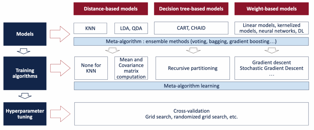
We will again use the same three-step framework to keep the explanation consistent and intuitive.
 Three learning steps in Machine Learning - Image by author
1. Base model
we will use decision tree regressors as our base model.
A decision tree is non-linear by construction. It splits the feature space into regions and assigns a constant prediction to each region.
An important point is that when trees are added together, they do not collapse into a single tree.
Each new tree introduces additional structure to the model.
This is where Gradient Boosting becomes particularly powerful.
1 bis. Ensemble model
Gradient Boosting is the mechanism used to aggregate these base models into a single predictive model.
2. Model fitting
For clarity, we will use decision stumps , meaning trees with a depth of one and a single split.
Each tree is trained to predict the residuals of the previous model.
2 bis. Ensemble learning
The ensemble itself is built using gradient descent in function space.
Here, the objects being optimized are not parameters but functions , and those functions are decision trees.
3. Model tuning
Decision trees have several hyperparameters, such as:
- maximum depth
- minimum number of samples required to split
- minimum number of samples per leaf
In this article, we fix the tree depth to one.
At the ensemble level, two additional hyperparameters are essential:
- the learning rate
- the number of boosting iterations
These parameters control how fast the model learns and how complex it becomes.
2. Gradient Boosting Algorithm
The Gradient Boosting algorithm follows a simple and repetitive structure.
2.1 Algorithm overview
Here are the main steps of the Gradient Boosting algorithm
- Initialization
Start with a constant model. For regression with squared loss, this is the average value of the target.
- Residual computation
Compute the residuals between the current predictions and the observed values.
- Fit a weak learner
Train a decision tree regressor to predict these residuals.
- Model update
Add the new tree to the existing model, scaled by a learning rate.
- Repeat
Iterate until the chosen number of boosting steps is reached or the error stabilizes.
2.2 Dataset
To illustrate the behavior of Gradient Boosted Trees, we will use several types of datasets that I generated:
- Piecewise linear data , where the relationship changes by segments
- Non-linear data , such as curved patterns
- Binary targets , for classification tasks
For classification, we will start with the squared loss for simplicity. This allows us to reuse the same mechanics as in regression. The loss function can later be replaced by alternatives better suited to classification, such as logistic or exponential loss.
These different datasets help highlight how Gradient Boosting adapts to various data structures and loss functions while relying on the same underlying algorithm.
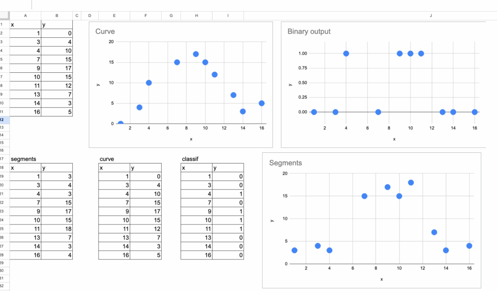 Datasets for Gradient Boosted Decision Tree Regressor - all image by author
2.3 Initialization
The Gradient Boosting process starts with a constant model.
For regression with squared loss, this initial prediction is simply the average value of the target variable.
This average value represents the best initial prediction before any structure is learned from the features.
It is also a good opportunity to recall: almost every regression model can be seen as an improvement over the global average.
- k-NN looks for similar observations, and predicts with the average value of their neighbors.
- Decision Tree Regressors split the dataset into regions and compute the average value within each leaf to predict for a new observation that falls into this leaf.
- Weight-based models adjust feature weights to balance or update the global average, for a given new observation.
Here, for gradient boosting, we also start with the average value. And then we will see how it will be progressively corrected.

2.4 First Tree
The first decision tree is then trained on the residuals of this initial model.
After the initialization, the residuals are just the differences between the observed values and the average.
 To build this first tree, we use exactly the same procedure as in the article on Decision Tree Regressors.
The only difference is the target: instead of predicting the original values, the tree predicts the residuals.
This first tree provides the initial correction to the constant model and sets the direction for the boosting process.

2.5 Model update
Once the first tree has been trained on the residuals, we can compute the first improved prediction.
The updated model is obtained by combining the initial prediction and the first tree’s correction:
f1(x) = f0 + learning_rate * h1(x)
where:
- f0 is the initial prediction, equal to the average value of the target
- h1(x) is the prediction of the first tree trained on the residuals
- learning_rate controls how much of this correction is applied
This update step is the core mechanism of Gradient Boosting.
Each tree slightly adjusts the current predictions instead of replacing them, allowing the model to improve progressively and remain stable.
2.6 Repeating the Process
Once the first update has been applied, the same procedure is repeated.
At each iteration, new residuals are computed using the current predictions, and a new decision tree is trained to predict these residuals. This tree is then added to the model using the learning rate.
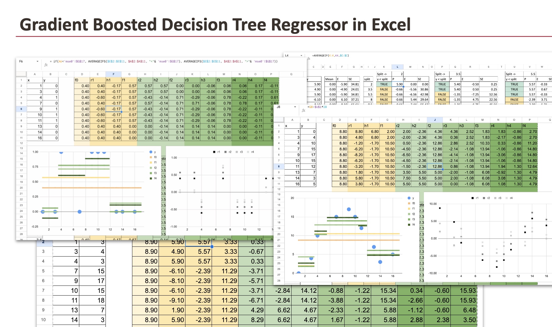
To make this process easier to follow in Excel, the formulas can be written in a way that is fully automated. Once this is done, the formulas for the second tree and all subsequent trees can simply be copied to the right.
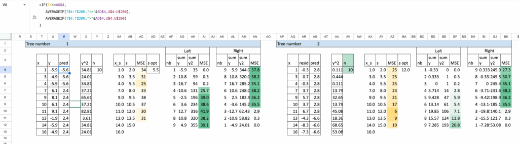 As the iterations progress, all the predictions of the residual models are grouped together. This makes the structure of the final model very clear.
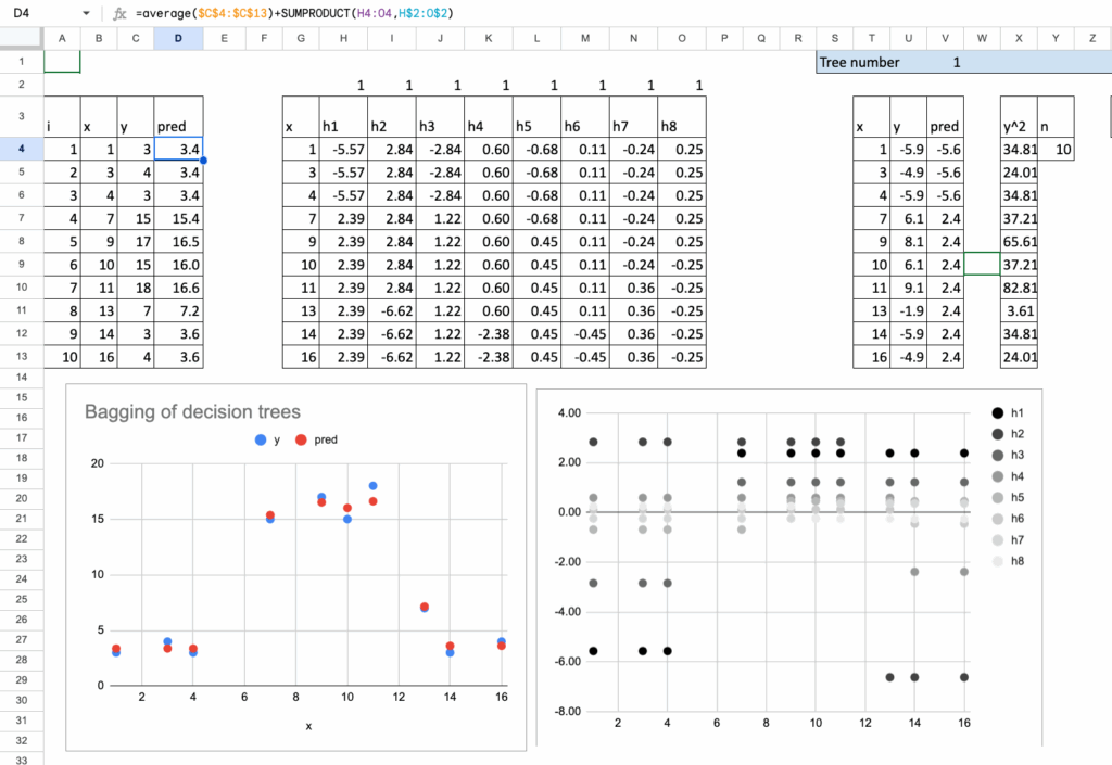
At the end, the prediction can be written in a compact form:
f(x) = f0 + eta * (h1(x) + h2(x) + h3(x) + ...)
This is one of those cases where details matter.
This representation highlights an important idea: the final model is simply the initial prediction plus a weighted sum of residual predictions.
It also opens the door to possible extensions. For example, the learning rate does not have to be constant. It can decrease over time, following a decay through the iteration process.
It is the same idea for the decay in gradient descent or stochastic gradient descent.
3. Understanding the Final Model
3.1 How the model evolves across iterations
We start with a piecewise dataset. In the visualization below, we can see all the intermediate models produced during the Gradient Boosting process.
First, we see the initial constant prediction , equal to the average value of the target.
Then comes f1 , obtained after adding the first tree with a single split.
Next, f2 , after adding a second tree, and so on.
Each new tree introduces a local correction. As more trees are added, the model progressively adapts to the structure of the data.
 The same behavior appears with a curved dataset. Even though each individual tree is piecewise constant, their additive combination results in a smooth curve that follows the underlying pattern.
 When applied to a binary target , the algorithm still works, but some predictions can become negative or greater than one. This is expected when using squared error loss, which treats the problem as regression and does not constrain the output range.
If probability-like outputs are required, a classification-oriented loss function, such as logistic loss, should be used instead.
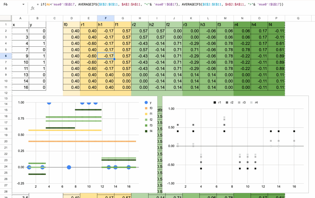 In conclusion, Gradient Boosting can be applied to different types of datasets , including piecewise, non-linear, and binary cases. Regardless of the dataset, the final model remains piecewise constant by construction , since it is built as a sum of decision trees.
However, the accumulation of many small corrections allows the overall prediction to closely approximate complex patterns.
3.2 Comparison with a single decision tree
When showing these plots, a natural question often arises:
Does Gradient Boosting not end up creating a tree, just like a Decision Tree Regressor?
This impression is understandable, especially when working with a small dataset. Visually, the final prediction can look similar, which makes the two approaches harder to distinguish at first glance.
However, the difference becomes clear when we look at how the splits are computed.
A single Decision Tree Regressor is built through a sequence of splits. At each split, the available data is divided into smaller subsets. As the tree grows, each new decision is based on fewer and fewer observations, which can make the model sensitive to noise.
Once a split is made, data points that fall into different regions are no longer related. Each region is treated independently, and early decisions cannot be revised.
Gradient Boosted Trees work in a completely different way.
Each tree in the boosting process is trained using the entire dataset. No observation is ever removed from the learning process. At every iteration, all data points contribute through their residuals.
This changes the behavior of the model fundamentally.
A single tree makes hard, irreversible decisions. Gradient Boosting, on the other hand, allows later trees to correct the mistakes made by earlier ones.
Instead of committing to one rigid partition of the feature space, the model progressively refines its predictions through a sequence of small adjustments.
This ability to revise and improve earlier decisions is one of the key reasons why Gradient Boosted Trees are both robust and powerful in practice.
3.3 General comparison with other models
Compared to a single decision tree , Gradient Boosted Trees produce smoother predictions, reduce overfitting, and improve generalization.
Compared to linear models , they naturally capture non-linear patterns, automatically model feature interactions, and require no manual feature engineering.
Compared to non-linear weight-based models , such as kernel methods or neural networks, Gradient Boosted Trees offer a different set of trade-offs. They rely on simple, interpretable building blocks, are less sensitive to feature scaling, and require fewer assumptions about the structure of the data. In many practical situations, they also train faster and require less tuning.
These combined properties explain why Gradient Boosted Decision Tree Regressors perform so well across a wide range of real-world applications.
Conclusion
In this article, we showed how Gradient Boosting builds powerful models by combining simple decision trees trained on residuals. Starting from a constant prediction, the model is refined step by step through small, local corrections.
We saw that this approach adapts naturally to different types of datasets and that the choice of the loss function is essential, especially for classification tasks.
By combining the flexibility of trees with the stability of boosting, Gradient Boosted Decision Trees achieve strong performance in practice while remaining conceptually simple and interpretable.
A note on learning order
Gradient Boosting is often presented as the most powerful ensemble method, and it is indeed very popular in practice.
However, understanding ensemble learning does not start with Boosting.
Bagging remains a simpler and more fundamental approach, especially from a statistical point of view.
It makes variance reduction explicit and offers useful insight into prediction uncertainty, which complements the optimization perspective of Gradient Boosting.
···
All the Excel files are available through this Kofi link. Your support means a lot to me. The price will increase during the month, so early supporters get the best value.
 All Excel/Google sheet files for ML and DL
Register Now to Continue Reading
Unlock Towards Data Science with a Free Account
All articles on Towards Data Science are available to registered users. Create a free account today to access this article and thousands more.
Register for freeSign in to your account
 Written By
See all from Angela and Kezhan Shi
AlgorithmsArtificial IntelligenceData ScienceDecision TreeGradient Boosting
Share This Article
Towards Data Science is a community publication. Submit your insights to reach our global audience and earn through the TDS Author Payment Program.
Write for TDS
Related Articles
Artificial Intelligence
Deep Dive into Multi-Head Attention, the secret element in Transformers and LLMs. Let's explore its math, and build it from scratch.
Cristian Leo
July 16, 202416 min read
Artificial Intelligence
Understanding the limits of deep learning and the quest for true continual adaptation
Salvatore Raieli
September 6, 202414 min read
Programming
What's the difference between distinct() and dropDuplicates() in Spark?
Giorgos Myrianthous
February 21, 20213 min read
Artificial Intelligence
A tour of infamous machine learning blunders and failures that caught the world's attention
Kenneth Leung
August 19, 20237 min read
Machine Learning
A side-by-side CNN implementation and comparison
Mike Cvet
March 8, 20249 min read
Machine Learning
Transforming property management with advanced analytics and machine learning models
Hans Christian Ekne
November 30, 201810 min read
Programming
Discussing how to select multiple columns from a DataFrame in pandas
Giorgos Myrianthous
September 1, 20214 min read
Machine Learning
Data scientists tell stories through data. But what stories can data tell about data scientists?
Éverton Bin
November 10, 20205 min read
Data Science
Modeling the spread of COVID using a spatial model in Python's Mesa library and visualization modules
Bassel Karami
November 30, 20213 min read
Your home for data science and AI. The world's leading publication for data science, data analytics, data engineering, machine learning, and artificial intelligence professionals.
Subscribe to Our NewsletterWrite For TDS•About•Advertise•Privacy Policy•Terms of Use
© Insight Media Group, LLC 2026•The New Stack•roadmap.sh•Creator Network
Recommended Articles
Close