Understanding normalization, linear layers, GELU activation, and how they work together inside GPT’s main processing unit
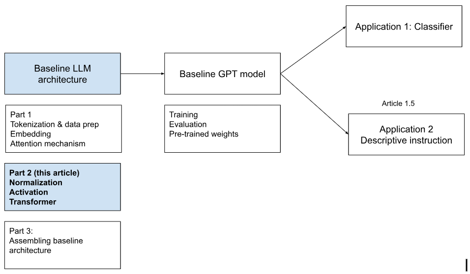
In the previous article, we looked at tokenization and embeddings, which convert a finite vocabulary into continuous vectors that we can work with mathematically. We also explored attention, which helps the model understand how different tokens relate to and influence one another in context.
In this article, we will look at a few more building blocks of a GPT-style model: normalization, linear layers, and activation functions. We will then bring them together inside the transformer block—the main processing unit that GPT repeats throughout the model.
At its simplest, normalization is about putting different numerical features onto a more consistent scale so they can be compared or combined more meaningfully.
Imagine ranking football players using three features:
Goals scored
Assists
Pass-completion rate
These values naturally live on different scales, so simply adding the raw numbers together would not tell us much.
One way to solve this is to normalize each feature. For goals, we could look at the minimum and maximum scored during a tournament and convert each player’s performance into a score between 0 and 1. We could then do the same for assists and pass-completion rate.
Instead of directly comparing 20 goals, 8 assists, and 90% pass completion, we would now have three scores on a common scale.
This football example uses min-max normalization. Layer normalization uses a different mathematical method, but the underlying motivation is similar: keeping values on a well-behaved scale.
In a GPT-style model, each token is represented by hundreds of numbers across its embedding dimensions. You can loosely think of these dimensions as the model’s internal features for representing that token.
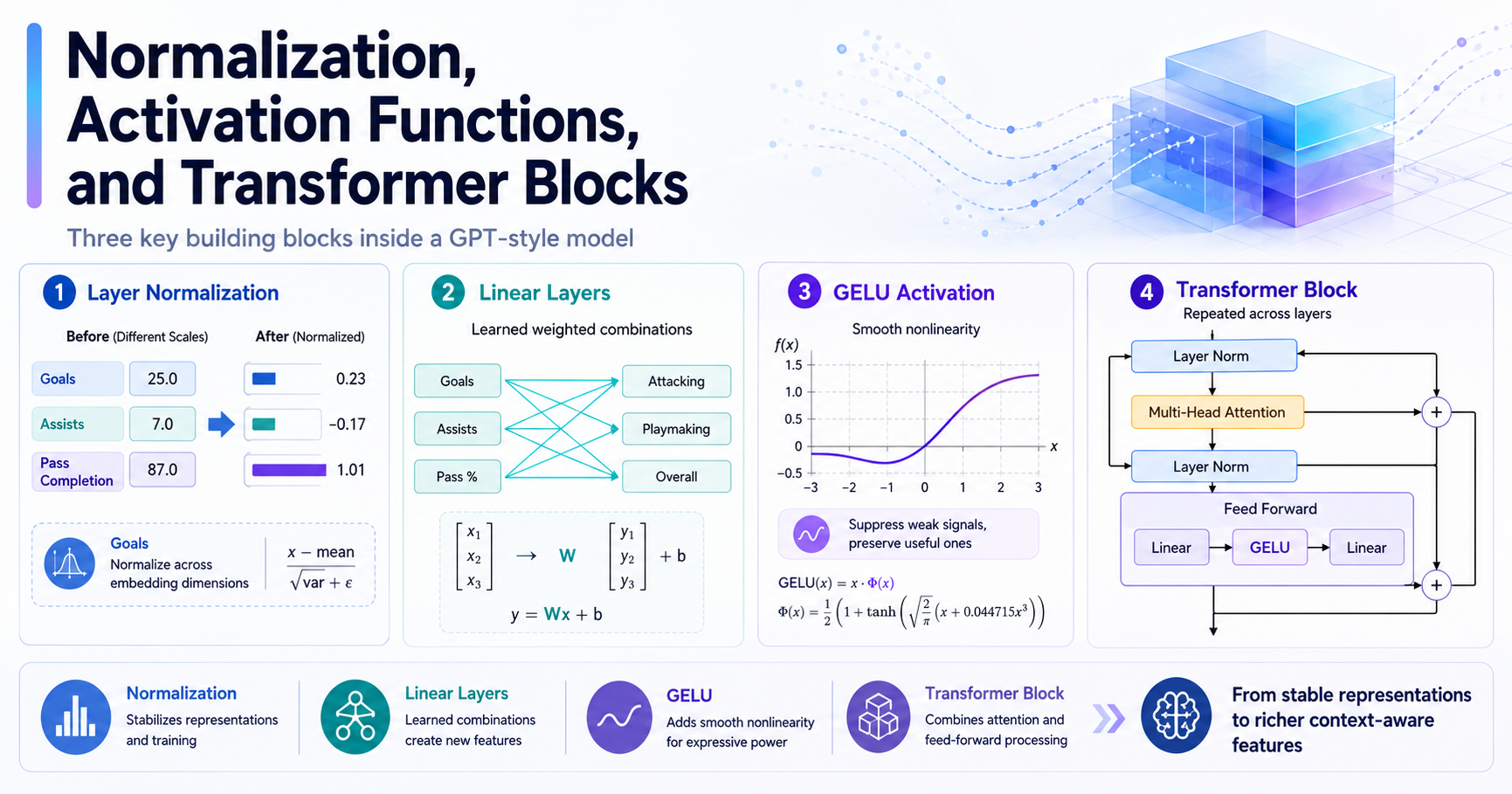
Layer normalization works on each token independently and normalizes across these embedding dimensions.
class LayerNorm(nn.Module):
    def __init__(self, emb_dim):
        super().__init__()
        self.eps = 1e-5
        self.scale = nn.Parameter(torch.ones(emb_dim))
        self.shift = nn.Parameter(torch.zeros(emb_dim))

    def forward(self, x):
        mean = x.mean(dim=-1, keepdim=True)
        var = x.var(dim=-1, keepdim=True, unbiased=False)

        norm_x = (x - mean) / torch.sqrt(var + self.eps)

        return self.scale * norm_x + self.shift
Here, dim=-1 tells PyTorch to calculate the mean and variance across the final dimension—the embedding dimension. It does not normalize across different tokens or across the batch.
The small eps value prevents division by zero, while scale and shift are trainable parameters. They allow the model to adjust the normalized values rather than forcing every representation to remain at exactly the same scale.
Why does this matter?
As token representations move through different model layers, their values can drift and end up on very different scales. Layer normalization acts as a kind of numerical housekeeping, bringing each token’s representation back into a more predictable range before the next major transformation.
We use normalization frequently inside a GPT model. Within every transformer block, token representations are normalized before the attention mechanism and again before the feed-forward network. After the full stack of transformer blocks, GPT-2 also applies one final normalization layer.
Exactly where normalization appears is an architectural design choice. Some transformer architectures place it before the major sub-layers, while others place it afterward.
The GPT-style architecture we are building uses pre-layer normalization, meaning normalization happens before attention and before the feed-forward network.
At a high level, a linear layer takes a set of input values and transforms them into a new set of values by combining the inputs with different weights.
Continuing our sports analogy, suppose we start with three features for scouting football players:
Goals
Assists
Pass-completion rate
We may want to transform them into three different scores:
Attacking ability
Playmaking ability
Overall contribution
Each score uses the same inputs, but with different weights. For example:
Attacking ability = 0.8 × goals score + 0.4 × assists score
+ 0.1 × passing score

Playmaking ability = 0.2 × goals score + 0.6 × assists score
+ 0.8 × passing score

Overall contribution = 0.4 × goals score + 0.4 × assists score + 0.6 × passing score
A GPT model does something similar.
The same token representation needs to be interpreted differently at different stages of the network. Linear layers create these new views by learning different weighted combinations of the existing representation.
Importantly, the weights inside a linear layer are trainable parameters. During training, the model continually adjusts them to learn which combinations of features are useful.
We already saw linear layers inside the attention mechanism, where separate projections transform the same token representation into queries, keys, and values.
They appear again inside the feed-forward network, where the representation is expanded into a larger intermediate space and then brought back to its original embedding size.
There is an important limitation to linear layers: stacking them alone does not make the network much more expressive.
Without an activation function between them, multiple linear transformations can effectively collapse into a single linear transformation. Activation functions introduce nonlinearity, allowing the model to learn much richer patterns.
Intuitively, a useful activation function should:
Introduce nonlinearity
Reduce weaker or less useful signals
Preserve sufficiently strong signals
Support stable learning through useful gradients
Our GPT model uses GELU, or the Gaussian Error Linear Unit:
class GELU(nn.Module):
    def __init__(self):
        super().__init__()

    def forward(self, x):
        return 0.5 * x * (
            1 + torch.tanh(
                torch.sqrt(torch.tensor(2.0 / torch.pi))
                * (x + 0.044715 * torch.pow(x, 3))
            )
        )
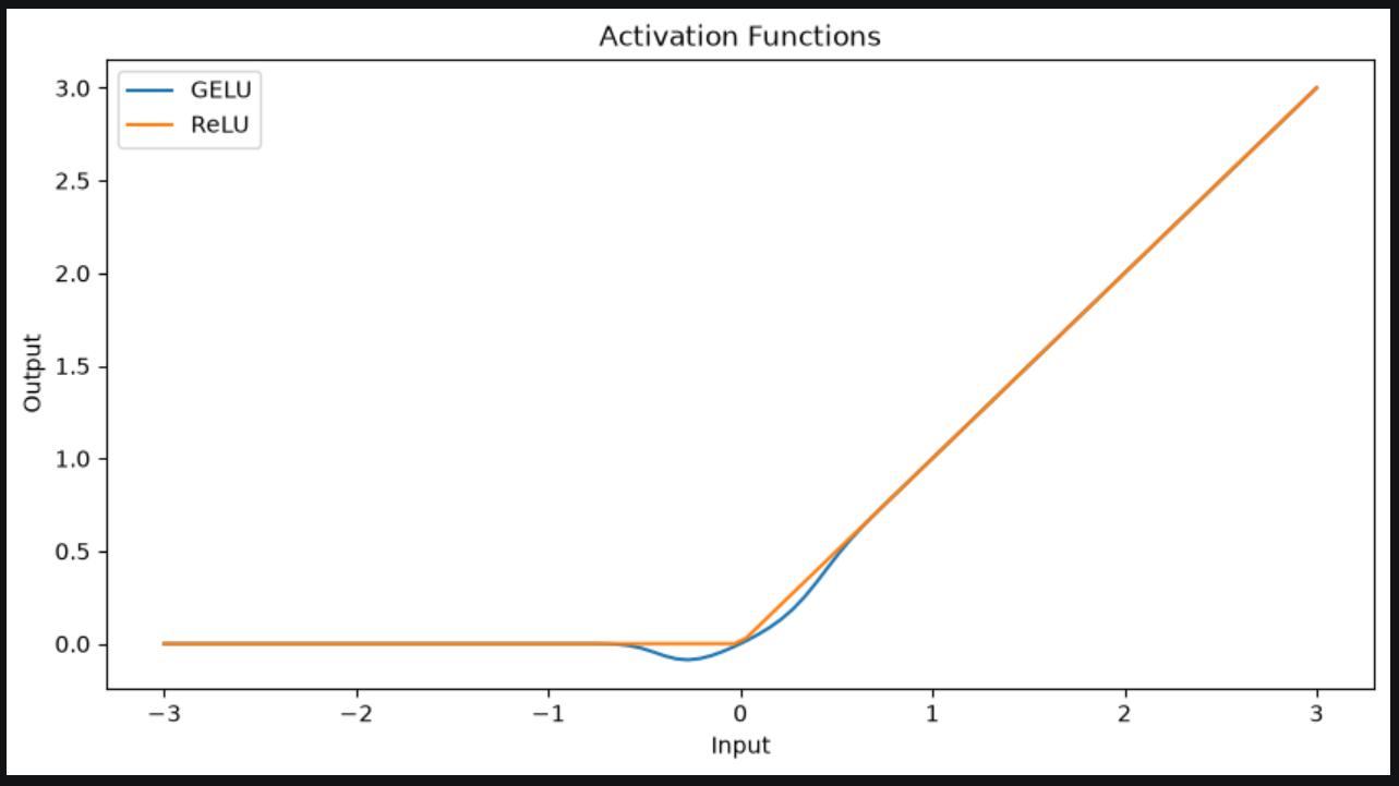
Unlike ReLU, which completely removes negative values, GELU applies a smoother filter.
Strong positive activations mostly pass through, strongly negative ones are largely suppressed, and values close to zero are only partially retained. This gives the model a more gradual way to decide which signals are useful.
Inside the GPT-2 feed-forward network, GELU sits between two linear layers:
self.layers = nn.Sequential(
    # Expand and then reduce the embedding dimensions
    nn.Linear(cfg["emb_dim"], 4 * cfg["emb_dim"]),
    GELU(),
    nn.Linear(4 * cfg["emb_dim"], cfg["emb_dim"]),
)
The first linear layer expands each token representation into a higher-dimensional space. For GPT-2 124M, this means expanding from 768 dimensions to 3,072.
GELU then filters the resulting activations before the second linear layer projects them back to the original 768-dimensional embedding space.
I think of this as temporarily giving the model a larger workspace. It creates a wider set of candidate features, filters them through GELU, and then compresses the useful information back into the standard representation required by the rest of the model.
The size of this intermediate space is another architectural design choice. A wider layer gives the model more capacity, but it also increases the number of trainable parameters and the computational cost.
GPT-2 uses an intermediate dimension four times larger than the embedding dimension as a practical balance.
One important distinction is:
Attention allows information to move between tokens, while the activation processes each token independently.
We now have all the components required for a transformer block.
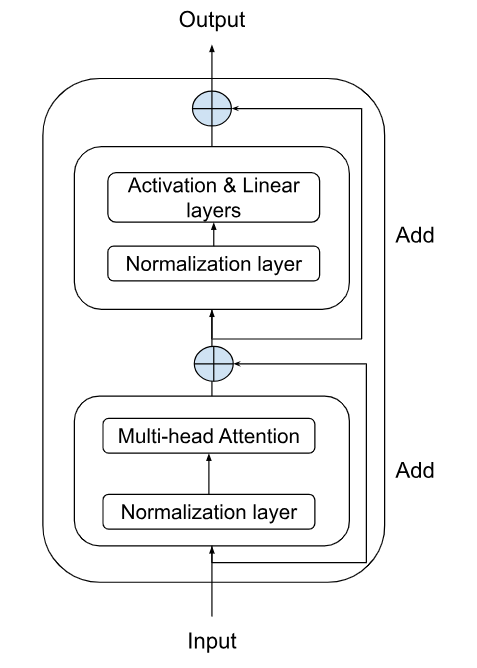
A transformer block is the main processing unit inside a GPT model. It helps each token gather relevant information from the sequence and then transforms the resulting representation into something richer.
Its overall flow looks like this:
Returning one final time to our sports analogy, we can think of each transformer block as another round of player evaluation.
The first normalization layer puts the player’s different features onto a stable numerical scale. Attention then evaluates the player in the context of teammates, opponents, and the wider game—not just through individual statistics.
The original player profile is added back through a shortcut connection, helping preserve the information we already had. The updated profile is then normalized again before entering the feed-forward network.
The feed-forward network reinterprets this updated profile. Its linear layers create new combinations of the available features, while GELU filters which signals should meaningfully influence the final assessment.
Another shortcut connection preserves the earlier representation instead of forcing every transformation to rebuild it from scratch.
In more technical terms, the sequence is:
Normalize the token representation.
Exchange information between tokens through attention.
Add back the original representation.
Normalize the updated representation.
Process each token independently through the feed-forward network.
Add back the representation from before the feed-forward network.
Note that we also have a Dropout layer after step 2 and step 4 - that drops randomly some information to prevent overfitting while training. I have removed this detail to keep it simple.
GPT-2 repeats this process across multiple transformer blocks. With every block, the representation of each token becomes more informed by both its own features and the context provided by the surrounding sequence.
At this point, we seem to have all the raw material needed for our GPT-2 model.
In the next article, we will assemble these components, walk through the end-to-end flow, and calculate how many trainable parameters we end up with.
Sebastian Raschka — Build a Large Language Model (From Scratch)
Vaswani et al. — Attention Is All You Need
Radford et al. — Language Models are Unsupervised Multitask Learners
Ba, Kiros, and Hinton — Layer Normalization
Xiong et al. — On Layer Normalization in the Transformer Architecture
Hendrycks and Gimpel — Gaussian Error Linear Units (GELUs)
Aman Jain — Project repository. The code and notebooks accompanying this learning journey are available on my GitHub profile.