保留正文与补采附件。源页面当前未重新核验;具体限制见交付清单。
 We value your privacy
We use cookies to enhance your browsing experience, serve personalised ads or content, and analyse our traffic. By clicking "Accept All", you consent to our use of cookies.
Customise Reject All Accept All
Customise Consent Preferences
 We use cookies to help you navigate efficiently and perform certain functions. You will find detailed information about all cookies under each consent category below.
The cookies that are categorised as "Necessary" are stored on your browser as they are essential for enabling the basic functionalities of the site. ... Show more
NecessaryAlways Active
Necessary cookies are required to enable the basic features of this site, such as providing secure log-in or adjusting your consent preferences. These cookies do not store any personally identifiable data.
-
Cookie
BCTempID
-
Duration
10 minutes
-
Description
No description available.
-
Cookie
__cf_bm
-
Duration
1 hour
-
Description
This cookie, set by Cloudflare, is used to support Cloudflare Bot Management.
-
Cookie
AWSALBCORS
-
Duration
7 days
-
Description
Amazon Web Services set this cookie for load balancing.
-
Cookie
_cfuvid
-
Duration
session
-
Description
Cloudflare sets this cookie to track users across sessions to optimize user experience by maintaining session consistency and providing personalized services
-
Cookie
li_gc
-
Duration
6 months
-
Description
Linkedin set this cookie for storing visitor's consent regarding using cookies for non-essential purposes.
-
Cookie
__hssrc
-
Duration
session
-
Description
This cookie is set by Hubspot whenever it changes the session cookie. The __hssrc cookie set to 1 indicates that the user has restarted the browser, and if the cookie does not exist, it is assumed to be a new session.
-
Cookie
__hssc
-
Duration
1 hour
-
Description
HubSpot sets this cookie to keep track of sessions and to determine if HubSpot should increment the session number and timestamps in the __hstc cookie.
-
Cookie
wpEmojiSettingsSupports
-
Duration
session
-
Description
WordPress sets this cookie when a user interacts with emojis on a WordPress site. It helps determine if the user's browser can display emojis properly.
-
Cookie
BCSessionID
-
Duration
1 year 1 month 4 days
-
Description
Blueconic sets this cookie as a unique identifier for the BlueConic profile.
-
Cookie
_octo
-
Duration
1 year
-
Description
No description available.
-
Cookie
logged_in
-
Duration
1 year
-
Description
No description available.
-
Cookie
__Secure-YEC
-
Duration
past
-
Description
YouTube sets this cookie to stores the user's video player preferences using embedded YouTube video
-
Cookie
__eoi
-
Duration
6 months
-
Description
Description is currently not available.
-
Cookie
AWSALBTGCORS
-
Duration
7 days
-
Description
No description available.
-
Cookie
login-status-p
-
Duration
past
-
Description
Description is currently not available.
-
Cookie
AWSALBTG
-
Duration
7 days
-
Description
No description available.
-
Cookie
csrf_token
-
Duration
session
-
Description
No description available.
-
Cookie
token_v2
-
Duration
1 day
-
Description
Description is currently not available.
-
Cookie
D
-
Duration
1 year
-
Description
Description is currently not available.
-
Cookie
PHPSESSID
-
Duration
session
-
Description
This cookie is native to PHP applications. The cookie stores and identifies a user's unique session ID to manage user sessions on the website. The cookie is a session cookie and will be deleted when all the browser windows are closed.
-
Cookie
VISITOR_PRIVACY_METADATA
-
Duration
6 months
-
Description
YouTube sets this cookie to store the user's cookie consent state for the current domain.
-
Cookie
cookietest
-
Duration
session
-
Description
The cookietest cookie is typically used to determine whether the user's browser accepts cookies, essential for website functionality and user experience.
-
Cookie
__Host-airtable-session
-
Duration
1 year
-
Description
This cookie is used to enable us to integrate the services of Airtable.
-
Cookie
__Host-airtable-session.sig
-
Duration
1 year
-
Description
This cookie is used to enable us to integrate the services of Airtable.
-
Cookie
m
-
Duration
1 year 1 month 4 days
-
Description
Stripe sets this cookie for fraud prevention purposes. It identifies the device used to access the website, allowing the website to be formatted accordingly.
-
Cookie
BIGipServer*
-
Duration
session
-
Description
Marketo sets this cookie to collect information about the user's online activity and build a profile about their interests to provide advertisements relevant to the user.
-
Cookie
__cfruid
-
Duration
session
-
Description
Cloudflare sets this cookie to identify trusted web traffic.
-
Cookie
_GRECAPTCHA
-
Duration
6 months
-
Description
Google Recaptcha service sets this cookie to identify bots to protect the website against malicious spam attacks.
-
Cookie
__Secure-YNID
-
Duration
6 months
-
Description
Google cookie used to protect user security and prevent fraud, especially during the login process.
-
Cookie
cookieyes-consent
-
Duration
1 year
-
Description
CookieYes sets this cookie to remember users' consent preferences so that their preferences are respected on subsequent visits to this site. It does not collect or store any personal information about the site visitors.
Functional
Functional cookies help perform certain functionalities like sharing the content of the website on social media platforms, collecting feedback, and other third-party features.
-
Cookie
lidc
-
Duration
1 day
-
Description
LinkedIn sets the lidc cookie to facilitate data center selection.
-
Cookie
brw
-
Duration
1 year
-
Description
No description available.
-
Cookie
brwConsent
-
Duration
5 minutes
-
Description
Description is currently not available.
-
Cookie
WMF-Uniq
-
Duration
1 year
-
Description
Description is currently not available.
-
Cookie
loom_anon_comment
-
Duration
1 year
-
Description
No description available.
-
Cookie
loom_referral_video
-
Duration
session
-
Description
Description is currently not available.
-
Cookie
VISITOR_INFO1_LIVE
-
Duration
6 months
-
Description
A cookie set by YouTube to measure bandwidth that determines whether the user gets the new or old player interface.
-
Cookie
yt-remote-connected-devices
-
Duration
Never Expires
-
Description
YouTube sets this cookie to store the user's video preferences using embedded YouTube videos.
-
Cookie
ytidb::LAST_RESULT_ENTRY_KEY
-
Duration
Never Expires
-
Description
The cookie ytidb::LAST_RESULT_ENTRY_KEY is used by YouTube to store the last search result entry that was clicked by the user. This information is used to improve the user experience by providing more relevant search results in the future.
-
Cookie
yt-remote-device-id
-
Duration
Never Expires
-
Description
YouTube sets this cookie to store the user's video preferences using embedded YouTube videos.
-
Cookie
yt-remote-session-name
-
Duration
session
-
Description
The yt-remote-session-name cookie is used by YouTube to store the user's video player preferences using embedded YouTube video.
-
Cookie
yt-remote-fast-check-period
-
Duration
session
-
Description
The yt-remote-fast-check-period cookie is used by YouTube to store the user's video player preferences for embedded YouTube videos.
-
Cookie
yt-remote-session-app
-
Duration
session
-
Description
The yt-remote-session-app cookie is used by YouTube to store user preferences and information about the interface of the embedded YouTube video player.
-
Cookie
yt-remote-cast-available
-
Duration
session
-
Description
The yt-remote-cast-available cookie is used to store the user's preferences regarding whether casting is available on their YouTube video player.
-
Cookie
yt-remote-cast-installed
-
Duration
session
-
Description
The yt-remote-cast-installed cookie is used to store the user's video player preferences using embedded YouTube video.
-
Cookie
cp_session
-
Duration
3 months
-
Description
Codepen sets this cookie for Help systems found in the website.
-
Cookie
loid
-
Duration
1 year 1 month 4 days
-
Description
This cookie is set by the Reddit. The cookie enables the sharing of content from the website onto the social media platform.
Analytics
Analytical cookies are used to understand how visitors interact with the website. These cookies help provide information on metrics such as the number of visitors, bounce rate, traffic source, etc.
-
Cookie
__hstc
-
Duration
6 months
-
Description
Hubspot set this main cookie for tracking visitors. It contains the domain, initial timestamp (first visit), last timestamp (last visit), current timestamp (this visit), and session number (increments for each subsequent session).
-
Cookie
hubspotutk
-
Duration
6 months
-
Description
HubSpot sets this cookie to keep track of the visitors to the website. This cookie is passed to HubSpot on form submission and used when deduplicating contacts.
-
Cookie
_ga
-
Duration
1 year 1 month 4 days
-
Description
Google Analytics sets this cookie to calculate visitor, session and campaign data and track site usage for the site's analytics report. The cookie stores information anonymously and assigns a randomly generated number to recognise unique visitors.
-
Cookie
ga*
-
Duration
1 year 1 month 4 days
-
Description
Google Analytics sets this cookie to store and count page views.
-
Cookie
__Host-psifi.analyticsTrace
-
Duration
6 hours
-
Description
Description is currently not available.
-
Cookie
__Host-psifi.analyticsTraceV2
-
Duration
6 hours
-
Description
Description is currently not available.
-
Cookie
_gh_sess
-
Duration
session
-
Description
GitHub sets this cookie for temporary application and framework state between pages like what step the user is on in a multiple step form.
-
Cookie
YSC
-
Duration
session
-
Description
YSC cookie is set by Youtube and is used to track the views of embedded videos on Youtube pages.
-
Cookie
ajs_anonymous_id
-
Duration
1 year
-
Description
This cookie is set by Segment to count the number of people who visit a certain site by tracking if they have visited before.
-
Cookie
vuid
-
Duration
1 year 1 month 4 days
-
Description
Vimeo installs this cookie to collect tracking information by setting a unique ID to embed videos on the website.
Performance
Performance cookies are used to understand and analyse the key performance indexes of the website which helps in delivering a better user experience for the visitors.
-
Cookie
AWSALB
-
Duration
7 days
-
Description
AWSALB is an application load balancer cookie set by Amazon Web Services to map the session to the target.
-
Cookie
acq
-
Duration
past
-
Description
Description is currently not available.
-
Cookie
acq.sig
-
Duration
past
-
Description
Description is currently not available.
-
Cookie
ptc
-
Duration
2 years
-
Description
No description available.
Advertisement
Advertisement cookies are used to provide visitors with customised advertisements based on the pages you visited previously and to analyse the effectiveness of the ad campaigns.
-
Cookie
muc_ads
-
Duration
1 year 1 month 4 days
-
Description
Twitter sets this cookie to collect user behaviour and interaction data to optimize the website.
-
Cookie
guest_id_marketing
-
Duration
1 year 1 month 4 days
-
Description
Twitter sets this cookie to identify and track the website visitor.
-
Cookie
guest_id_ads
-
Duration
1 year 1 month 4 days
-
Description
Twitter sets this cookie to identify and track the website visitor.
-
Cookie
personalization_id
-
Duration
1 year 1 month 4 days
-
Description
Twitter sets this cookie to integrate and share features for social media and also store information about how the user uses the website, for tracking and targeting.
-
Cookie
guest_id
-
Duration
1 year 1 month 4 days
-
Description
Twitter sets this cookie to identify and track the website visitor. It registers if a user is signed in to the Twitter platform and collects information about ad preferences.
-
Cookie
bcookie
-
Duration
1 year
-
Description
LinkedIn sets this cookie from LinkedIn share buttons and ad tags to recognize browser IDs.
-
Cookie
__Secure-ROLLOUT_TOKEN
-
Duration
6 months
-
Description
YouTube sets this cookie to manage feature rollout and experimentation. It helps Google control which new features or interface changes are shown to users as part of testing and staged rollouts, ensuring consistent experience for a given user during an experiment.
-
Cookie
yt.innertube::nextId
-
Duration
Never Expires
-
Description
YouTube sets this cookie to register a unique ID to store data on what videos from YouTube the user has seen.
-
Cookie
yt.innertube::requests
-
Duration
Never Expires
-
Description
YouTube sets this cookie to register a unique ID to store data on what videos from YouTube the user has seen.
-
Cookie
session_tracker
-
Duration
session
-
Description
This cookie is set by the Reddit. This cookie is used to identify trusted web traffic. It also helps in adverstising on the website.
-
Cookie
edgebucket
-
Duration
session
-
Description
Reddit sets this cookie to save the information about a log-on Reddit user, for the purpose of advertisement recommendations and updating the content.
-
Cookie
did
-
Duration
1 year
-
Description
Arbor sets this cookie to show targeted ads to site visitors.This cookie expires after 2 months or 1 year.
Uncategorised
Other uncategorised cookies are those that are being analysed and have not been classified into a category as yet.
No cookies to display.
Reject All Save My Preferences Accept All
Toggle SearchToggle Mobile Navigation
Publish AI, ML & data-science insights to a global community of data professionals.
Sign inSubmit an Article
LatestEditor's PicksNewsletterShipAI
Write For TDS
LinkedInXToggle Search
Data Science
An Introduction to Linear Regression
Regression is used primarily if you wish to predict or explain numeric data
James Andrew Godwin
March 8, 202119 min read
 Regression | Photo by Hao Wang
This article is a continuation of series that last covered Bayes statistics.
Volatility is inherent within the stock market, but perhaps the rise of "meme stocks" is something that is beyond traditional comprehension. This article is not about such "stonks" - which is the ironic misspelling of stocks that encapsulates the new investing zeitgeist amongst Millennials (broadly speaking). Rather, I was pondering the fabulous rollercoaster of a ride of $GME as a timely example of something to apply linear regression to; one can apply a linear regression model to a given stock to predict its price in the future. This article and subsequent articles will expand upon the concepts of linear regression and several methods associated with it, its associated errors for model analysis as well as touching on residuals.
But what is regression? The goal of regression is to produce a model that represents the best fit for some observed data. A better, more specific way to state this is that regression is used to predict or explain numeric data **** - smarter people than me have been applying such models to financial data (like $GME) for decades. But, if you want to predict whether or not somebody is going to come down with a disease or whether or not somebody will be wearing black, or whether an asset will appreciate or depreciate in value those would not be regressions, those would be classifications. A** regression is either an explanatory model or a predictive model for numeric dat**a. And for the most part, we will be dealing with ones where we can describe a function - that means an output - we can describe the relationship between one or more input variables and a single output variable (for linear regression).
History
Regression is based on the method of least squares or the method of minimum mean square error. The ideas around least squares or averaging errors have evolved over nearly three centuries. The first known publication of a 'Method of Averages' was by the German astronomer Tobias Mayer in 1750. Pierre-Simon Laplace published in 1788 a similar method. The first publication of the method of least squares was by the French mathematician Adrien-Marie Legendre in 1805.
As a historical aside, it is very likely that the German physicist and mathematician Carl Friedrich Gauss developed the method of least-squares as early as 1795, but he did not publish this method until 1809. Legendre firmly opposed any notion that Gauss had used the method earlier than the 1805 publishing date.
Francis Galton, a cousin of Charles Darwin, coined the term regression in 1886. Galton was interested in determining which traits of plants and animals, including humans, could be said to be inherited. While Galton invented a modern form of regression, it was Karl Pearson who put regression and multiple regression on a firm mathematical footing. He created the world's first university statistics department at UCL. Pearson's 1898 publication proposed a method of regression as we understand it today.
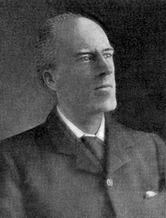 Karl Pearson | Source Wikipedia
Numerous others have expanded the theory of regression over the last century since Pearson's pivotal paper. Notably, Joseph Berkson published the logistic regression method in 1944, one of the first classification algorithms. In recent times the explosion of interest in machine learning (ML) has lead to a rapid increase in the numbers and types of regression models.
Types of regression
There are a variety of types of regressions including many that are nonlinear and have absolutely nothing to do with what I will cover; they are used to predict numeric outcomes but use different underlying technologies. Some common regression types are:
- Linear - most common
- Logistic - binary outcomes (success/failure)
- Polynomial - when a straight line is not the best fit
- Stepwise Ridge, and Lasso (common in ML)
Least-squares linear regression
Least-squares regression is the type I will be expounding on today. Caution, most people will conflate this with linear regression. Now the two need not be the same, but just warning you that most people will conflate these two. Linear regression just means that you are going to do something using a linear collection of parameters. There are a variety of other ways to do regressions and those would not use those linear collections of parameters; where each parameter is associated with one variable.
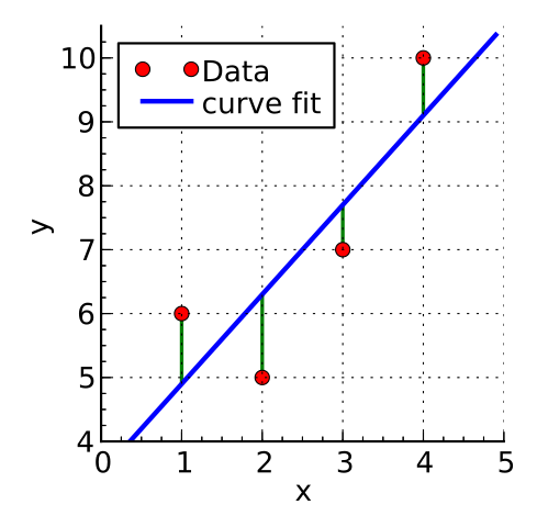 Linear Regression | Source Wikipedia
We have our linear regression, which is most commonly used to describe a straight line like the picture above - but that would also be true for logistic and polynomial. And probably also for most cases of a stepwise ridge and lasso. So there are two definitions of linear - and it will be confusing.
The one definition of linear is a line that goes through your data. Said another way, a line is fitted to your data. The other definition of linear is when you have a linear collection of parameters , with each parameter being associated with one variable. Said differently: the linearly predictable behavior of the dependent (target) value based on the explanatory variables.
This is a fancy way of saying:
 Linear collection of parameters
In the example above the parameters a, b, c have a linear association with the input variables x1, x2, and x3 - x0 is the offset. When I say variables, that means that they are inputs to a regression.
The least-squares linear regression was derived with the help of linear algebra and some calculus. I believe that understanding linear models is the basis for understanding the behavior of a whole bunch of statistical and ML models. In fact, I believe that about half of all machine learning models will use some of this form of linear regression, at least in their starting points.
Model selection: 11 dots
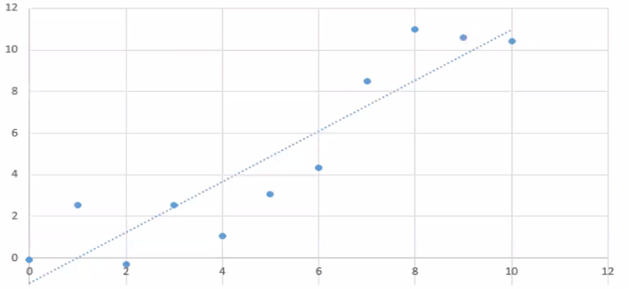 Model 1 | First-order linear regression, a simple line of best fit
A very reasonable and acceptable way to do a regression for some data (like the above example) is just to eyeball it and draw your line through it. And you want to call that a regression, that is fine. I doubt it can be called a linear regression anymore, but it is certainly a regression. And it is a very valid one. Now we are going to be talking about regressions where we can show mathematical rules for going from data points to a line of best fit.
 Mathematically defining the line above
Earlier I defined linear regression, now I will show an example of a quadratic equation that is still linear the way we have defined it:
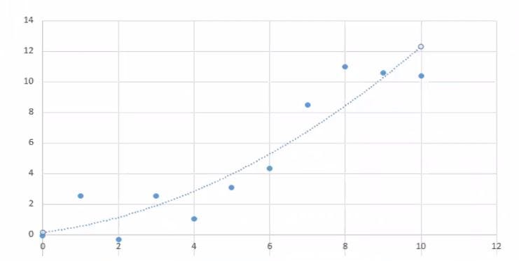 Model 2 | Quadratic regression of the second order
 equivalently:
 What we are going to do that or what we could do is we can say, "okay", y is not the output from a function that takes in one variable, namely x1, but rather y is the output from a function that takes in two variables; the first one being x1, the second one being x1². In fact, we can just call x1 times x1 the variable x2.
 By relabeling x1² as x2, we have recovered a linear regression
We can have non-straight lines fit a linear equation! Extending from this we can basically go to any polynomial. The following graph has the same data as the quadratic example, but a different line of best fit.
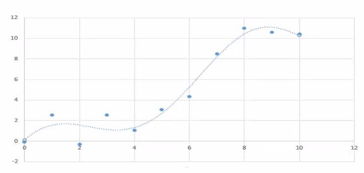 Model 3 | Higher-order regression using the same data as quadratic example
The only thing really changing is the line that we are drawing through them. In both cases, we are using what we call a linear relationship - well people who are in this regression business (mathematicians/physicists) call it such. They know full well that this is not a straight line. But they claim that in higher dimensions, this is actually straight; calling it not a line but a hyperplane.
The hyperplane is not curved in those dimensions. The dimensions would likely be:
 Maybe a fourth-order is needed.
This is adjacent to the mathematical field of topology, very relevant to particle physicists and Einstein's General Relativity, in general (haha)! Physicists will say that the path of a hit baseball is a straight line. In high school, we learned that this path is a parabola but in curved space-time, the path is a straight line geodesic (a geodesic being a "straight" line in a curved topological landscape). Geodesics you are likely familiar with include the lines of latitude on a globe.
So here the relevant question being asked is which of these three proceeding models is correct? The first order linear one? The second-order linear one? The fourth-order linear one? Well, the better question is which of these three is more useful, and that would naturally require that we have knowledge of what the model is being used for.
The general rule is, and this is a pretty important rule, that the simpler the model, the more useful it is. Remember this heuristic! Later I will write about regularization, which is just a way of making models simpler. When you simplify your linear model (well any model, but the context here is linear models) it is not just easier to understand, more importantly, they work better!
No data are perfect, errors will always exist. Another useful heuristic to remember is "all models are wrong, but some are useful!" The fact is that some of the data above could just be errors. The 11 dots above are the training data. When we look at new data, it might turn out, or probably will turn out, that they will not follow the funny curve, our higher-order model. Chances are that the "hyperplane" model is probably an example of what we call overfitting. And the reverse process of overfitting or the process that undoes overfitting is called regularization. As such, the balance of probability says that our first model is the most useful model to conduct further analysis on.
Terminology
- Response (Dependent) variable: the variable of primary interest, the variable we are trying to predict or explain. Like in our Jupyter notebook examples above, the response is the lefthand side of the equal sign -'y' is DEPENDENT on the values on the righthand side of the equals sign
- Explanatory (Independent) variable: the variable that attempts to explain the observed outcomes of the response variable. In an equation, if you change the 'y' (dependent) variable, you are not changing the righthand side 'x' variables - hence they are INDEPENDENT of changes in 'y'
There are two types of parameters in linear models:
- y-intercept, referred to above as the offset
- slope , rise over run, change in y divided by change in x. If there are multiple inputs, then we have multiple slopes (we call these partial slopes)
As an aside, but I want to mention that data is often not linear, and as such the data need to be transformed to apply regression analysis. An important such transformation is doing a log transformation when dealing with nonlinear data.
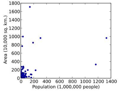 Country area vs population | Source Wikipedia
This raw data is not linear, however, we can make it appear linear by applying a logarithmic change, here it will be log base 10:
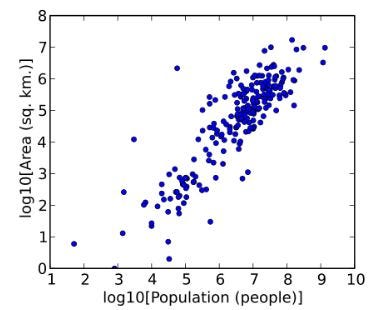 The same data, transformed | Source Wikipedia
The reason for doing the log transformation is because now your errors are going to probably be consistent throughout and that is very probably going to be better. It is possible to fit an exponential line to the data, doing non-parametric line fitting, but then the errors would not be consistent, they would not be of the same scale - which makes doing downstream analysis much harder.
Error terminology
Before explaining least-squares regression, we need to understand what the errors are:
 epsilon for error, i for which data point it is (first, second, etc.)
The E(error) is the distance between each point and the regression line. We select the line with the smallest sum of squared differences between each point and the line.
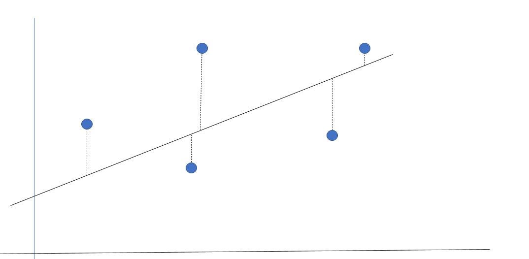 Regression line and errors for each point
The line above is a pretty good fit for the five dots above, but it is not perfect. What we want to know is how much error is there in the dependent variable. The epsilon term is added to bridge the gap between our predicted value(y_hat), which is where the red dot follows the green line and meets the regression line, and the actual observed values. The error is the difference between the predicted and observed variables. This is further explained in the code analysis below.
With a little bit of calculus and linear algebra, we try to find the minimum value of the sum of the errors for all possible regression lines. This summation is the best fit line. This is incredibly laborious to calculate. If instead, you say you want to minimize the square of this value, it turns out that there are beautiful, analytical solutions. And this is why we do least-squares fitting. So we do not try to minimize those dotted lines, or the sum of those dotted lines, we try instead to minimize the sum of the squares. So what is the sum of squares?
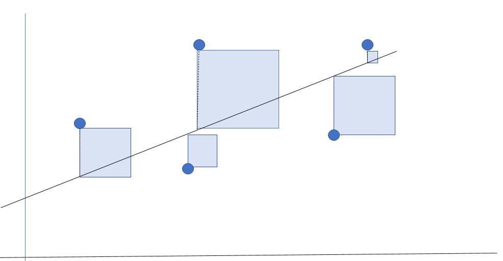 Visualization of the sum of squared errors for the regression line
The squares are now summed. The smallest total area of these squares is what we believe to be our best fit line. The advantage of this method, besides the beautiful analytical solutions, is that it penalizes larger errors - it punishes outliers. In the example above say that the largest error is 6 times larger than the smallest error. Well in least-squares regression that error is 36 (6 x 6)times more weighted than the smallest square.
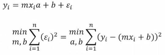 Explicit solutions exist using calculus
We let the computers solve the equation above to find the sum of least-squares by playing around with the slope and intercept. The predicted (theoretical) values are subtracted from the actual (observed) values and summed.
Python example: regression model
The following code can be run in a Jupyter Notebook to help get a feel and a visualization for least-squares linear regression.
N.B. we use synthetic data because we have a lot of control over what happens. Synthetic data is not always the best.
text
# relevant imports
import numpy as np
import pandas as pd
import matplotlib.pyplot as plt
%matplotlib inline
text
# synthetic data points between 0 and 10 with standard deviation of #the errors of 1 (std deviation of y should be around 3-the square #root of 10)
n_points = 80
x_start, x_end = 0, 10
y_start, y_end = 0, 10
y_sd = 1 # std deviation of the errors
text
# data columns, the y values are the errors added to the x values
x_data = np.linspace(x_start, x_end, n_points)
y_error = np.random.normal(loc=0, scale=y_sd, size=n_points)
y_data = np.linspace(y_start, y_end, n_points) + y_error
text
# create dataframe
syn_data = pd.DataFrame({'x':x_data, 'y':y_data})
text
syn_data.head()
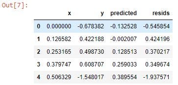
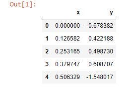 The first five lines of our 80 synthetic data points
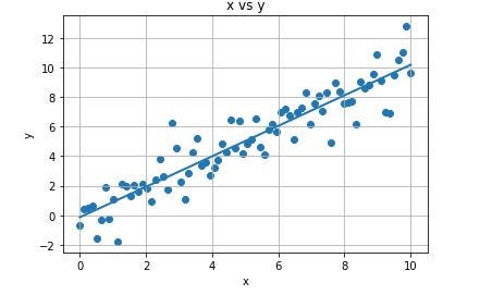
Let us now visualize the data - note the strong linearity of the data. Remember that the point of this exercise is to answer the question "if we know the value of X can we predict the value of Y?" We believe that by drawing the line of best fit that if someone gives us an X, say an X that we do not already have, then we can figure out what the Y value would be.
text
plt.plot(syn_data['x'], syn_data['y'], 'ko') # ko = black points
plt.grid(True)
plt.xlabel('x')
plt.ylabel('y')
plt.title('x vs y')
plt.show()
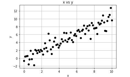 Our synthetic data - for the most part, the x values are approximately the y values
Building linear regression model
Following a simple template, we can build our model. You are likely familiar with one common package that can do this: Sci-Kit Learn. A quirk of sklearn is that works best with NumPy arrays, it is just what it is used to. The following template reshapes and converts the data for model training and evaluation:
text
# standard lin reg template
text
# imports
import numpy as np
import matplotlib.pyplot as plt
from sklearn.linear_model import LinearRegression
from sklearn.metrics import mean_squared_error, r2_score
text
# create numpy arrays for the x (independent) and y (dependent) #variables
x = syn_data.x.values.reshape(-1,1)
y = syn_data.y.values.reshape(-1,1)
text
# model initialization
regression_model = LinearRegression()
text
# train the model (fit data)
regression_model.fit(x, y)

y_predicted = regression_model.predict(x)
text
# model evaluation
rmse = mean_squared_error(y, y_predicted)
r2 = r2_score(y, y_predicted)
text
# printing values
print('Slope:' ,regression_model.coef_)
print('Intercept:', regression_model.intercept_)
print('Root mean squared error: ', rmse)
print('R2 score: ', r2)
text
# plotting values
plt.scatter(x, y, s=10)
plt.xlabel('x')
plt.ylabel('y')
text
plt.plot(x, y_predicted, color='r')
plt.show()
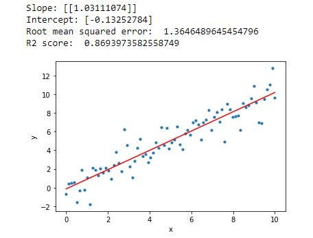 The line is a good fit for the data
The statistical values are explained in greater detail below when we evaluate the model's performance.
Plot residuals
The following is an important tool in understanding how good your regression model is - a residual plot. What is happening is that for every point, the difference between the observed and predicted values is plotted.
text
import seaborn as sns
sns.residplot(x, y)
plt.show()
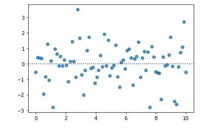 The predicted y value differences from actual y values
The residuals are the errors, which we plotted earlier. The x-axis is the x values. The y axis is the discrepancy between the actual y values and the predicted y values, the errors.
text
from sklearn import linear_model
# from sklearn.linear_model import LinearRegression
text
# initialize the model.
linear_model = linear_model.LinearRegression()
text
# define x and y
x_input = syn_data['x'].values.reshape(n_points, 1)
y_output = syn_data['y'].values.reshape(n_points, 1)
text
# fit the model to the existing data with lm.fit(x,y)
linear_model.fit(x_input, y_output)
text
# fit model to make predictions
y_pred = linear_model.predict(x_input)
text
# plot
plt.scatter(x_input, y_output)
plt.plot(x_input, y_pred, linewidth=2)
plt.grid(True)
plt.xlabel('x')
plt.ylabel('y')
plt.title('x vs y')
plt.show()
text
# model parameters
print('Intercept: {0:.5f}'.format(linear_model.intercept_[0]))
print('Slope : {0:.5f}'.format(linear_model.coef_[0][0]))
Stats Model package
Another, older and lesser-used Python package is Stats Model sm. The following code duplicates the Sci-Kit Learn work. Note the subtle differences between the two w/r to how the outputs are displayed.
N.B. The statistics are the same, but the presentations and the robustness thereof differ between the packages. sklearn is the preferred package to learn these days.
text
import statsmodels.formula.api as sm
text
# ols = ordinary least squares
ols_model = sm.ols(formula = 'y ~ x', data=syn_data)
text
# fit the model
results = ols_model.fit()
text
print('Intercept: {0:.5f}'.format(results.params.Intercept))
print('Slope : {0:.5f}'.format(results.params.x))
 text
# add predicted to dataframe
syn_data['predicted'] = y_pred
text
# add residuals to dataframe
syn_data['resids'] = y_output - y_pred
text
# verify data is as expected
syn_data.head()
 text
# coefficients of line of best fit
m = linear_model.coef_[0]
b = linear_model.intercept_
print('m = {}'.format(m[0]))
print('b = {}'.format(b[0]))

Interpreting the parameters
It is very important to know how to interpret the parameters (your results will be different because of the random seed in creating the data).
- y-intercept (b) : when x is zero, y is -0.13...
- slope (m) : When we increase x by 1 then we expect that y will go up by 1.03....
Simple enough, I bet most readers will have a strong grasp on these basics, but it is important to refresh everyone and to build up from a solid and universal foundation.
Model summary statistics
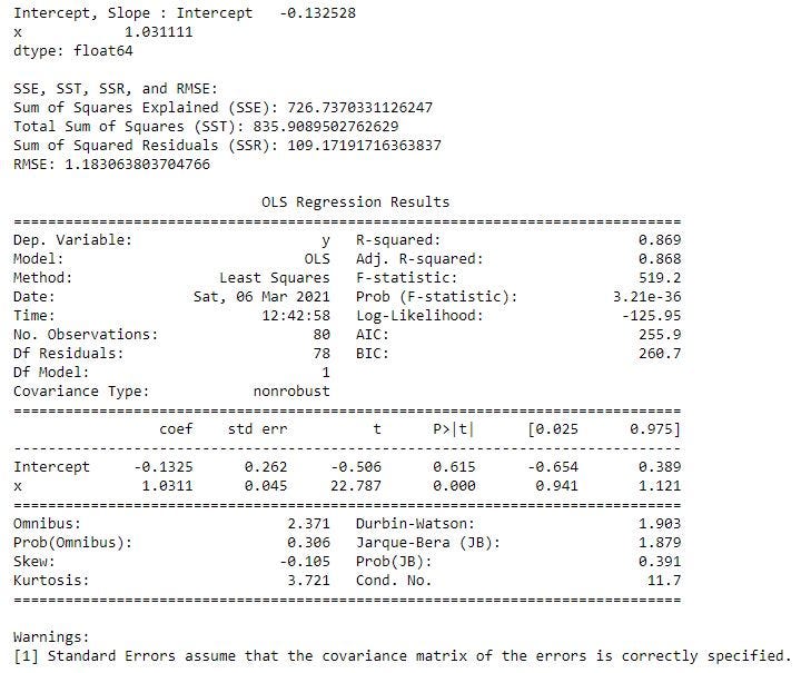
This is where SM shines - the beautiful results summary. A lot more data is shown natively than we need to understand least - squares regression at the moment. The residuals are also plotted after the OLS report.
text
import statsmodels.formula.api as sm
import seaborn as sns
text
ols_model = sm.ols(formula = 'y ~ x', data=syn_data)
text
results = ols_model.fit()
text
# print slope (m) and y-intercept (b)
print('Intercept, Slope : {}'.format(results.params))
text
print('nSSE, SST, SSR, and RMSE:')
mean_y = np.mean(y_output)
sst = np.sum((y_output - mean_y)**2)
ssr = np.sum((y_pred - y_output)**2)
sse = np.sum((y_pred - mean_y)**2)
text
print('Sum of Squares Explained (SSE): {}'.format(sse))
print('Total Sum of Squares (SST): {}'.format(sst))
print('Sum of Squared Residuals (SSR): {}'.format(ssr))
print('RMSE: {}'.format(np.sqrt(results.mse_resid)))
text
# print linear regression statistics
print('n', results.summary())
 text
# plot histogram of the residuals
sns.distplot(results.resid, hist=True)
plt.xlabel('Residual')
plt.ylabel('Frequency')
plt.title('Residual Histogram')
plt.show()
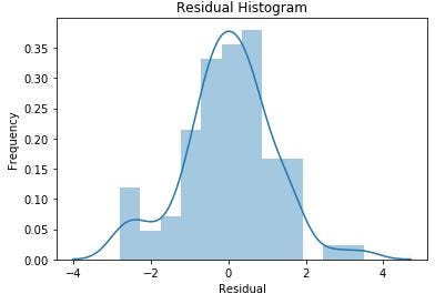 The first thing to note about our residuals plotted above is that they are roughly normal. This is to be expected because the synthetic data was created to be such, so this a bit of a self-fulfilling prophecy. The y data is created from errors added to the randomly generated x data, with the y data having a standard deviation of +/- one.
Evaluation of regression models
Now that we have built a regression model, we can quantitatively evaluate the performance of our regression model. The evaluation of regression models is based on measurements of the errors.
If we want to know how well we did, we must consider what a good benchmark would be. A common easy benchmark is to see if we can predict better than just the mean of the target variable.
We define the following terms:


 Now we need to define the following error metrics:
- Sum of Squared Residuals (SSR) : This is the value that the method of least squares was able to minimize to with the best fit line. The goal of regression is to minimize this quantity.
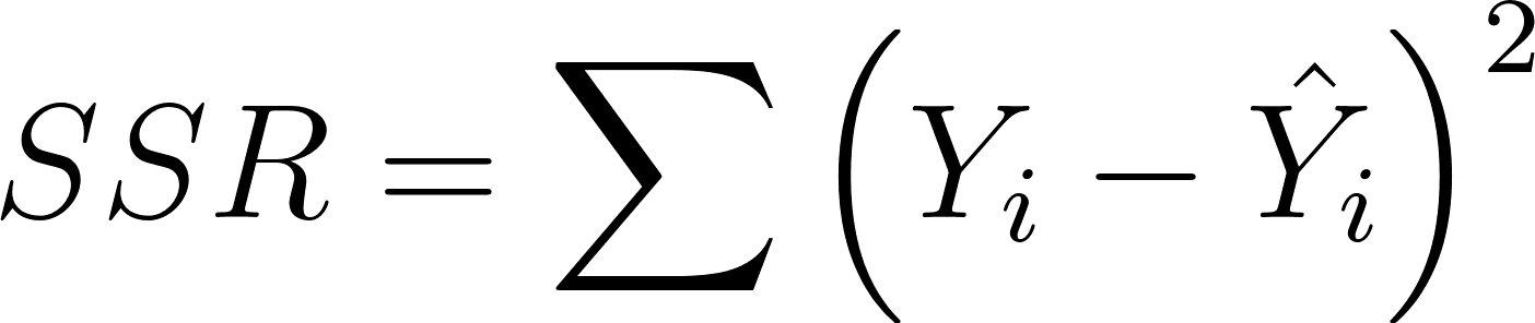 The goal of regression - minimize this
- Sum of Squared Total (SST) : This is a measure of how bad a prediction the target-mean would be

- Sum of Squared Explained (SSE) : This is a sum of a squared pointwise difference of the (SST - SSR). You can also think of this as a measurement of how much better we are explaining the variation than the mean
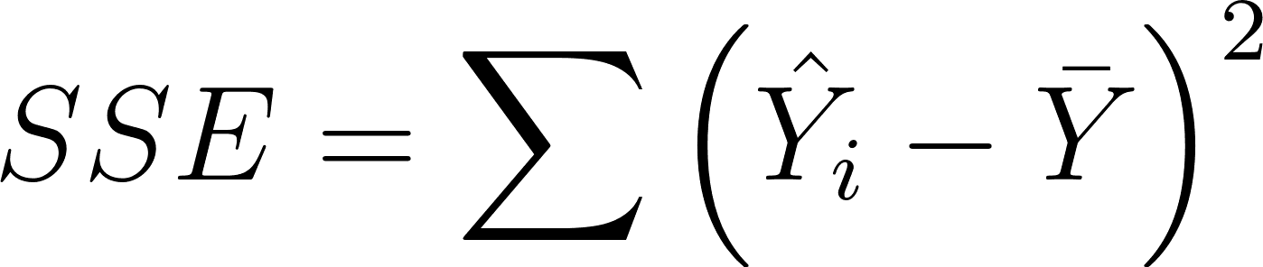 Notice that SST = SSR + SSE
- This formula is only true if you do your regression on your training data! If you do it on test data, this formula is no longer true. This formula is true for the cases where your coefficient of determination (COD)is the same as your Pearson's R², the correlation coefficient. They are not the same! They can sometimes be the same, but only in the situation for at least-squares fitting on your training data, not for when you use either your test data or not when you do a non least-squares fitting. SSR can become larger than SST, leading to a negative R²!
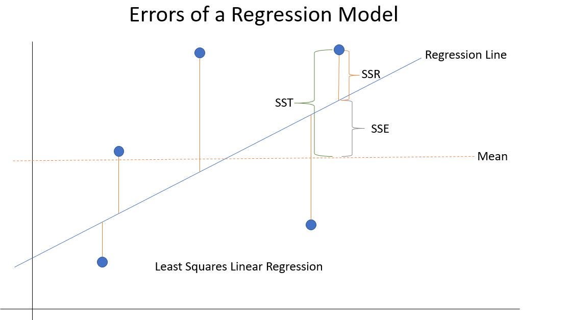 Visualization of the errors of a linear regression model
We can now talk about the Root-Mean-Squared-Error (RMSE). The reason we do this is that the "sum-squared-error" (also referred to as the mean-squared error) is in units of x². To convert the error to units of x , we need the square root of the mean-squared-error or the square root of the sum-squared residuals. This is the RMSE:
 Remember that the goal of regression is to minimize the residual error, SSR. Specifically, we wish to explain the maximum amount of the variance in the original data as possible with our model. We can quantify this idea with the coefficient of determination (COD)also known as R² :
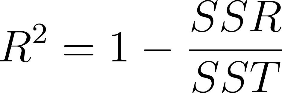 ONLY CORRECT WITH LEAST-SQUARES FITTING AND MEASURING TRAINING DATA
so as

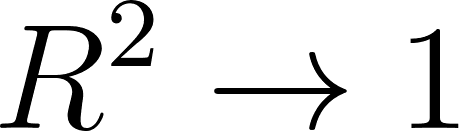 R² is the fraction of the variance of the original data explained by the model. A model that perfectly explains the data has R² = 1. A model which does not explain the data at all has R² = 0. This means that the training data is spread out so evenly that you cannot draw any best fit line through it. You can draw a line through the data, it just would not be the best fit line.
However, R² is not perfect:
- R² is not bias adjusted for degrees of freedom
- More importantly, there is no adjustment for the number of model parameters. As the number of model parameters increases, SSR will generally decrease. Without an adjustment, you will get a false sense of model performance
We address this by defining Adjusted R² (R² adj) :
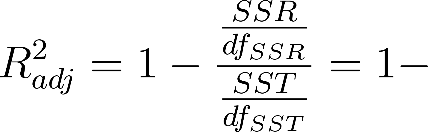
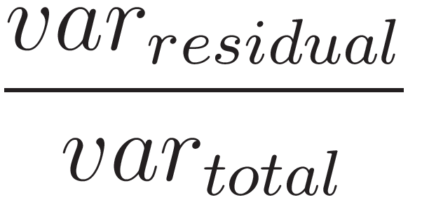 where

 This gives R²adj as:
 where

 Which can be rewritten:
 Now we have a metric that decreases with more added parameters, rewarding simplicity - remembering from earlier that simpler models are preferred to complex models.
Conclusion
We have covered many regression concepts so far:
- The single regression equation of a line is
- Use the Python model object
linear_model.LinearRegression() to initialize the model
- Use the
fit method to fit the model to the data
- Use
predict method to compute scores(predict values) for the dependent value (y)
- Pull the model parameters - m(slope) with
coef and b(y-intercept) - with intercept
- The residuals are the difference between the y_output and the y_predicted
- Use the
statsmodels and seaborn libraries to get summary statistics and make diagnostic plots
sklearn is preferable to the sm package, it is simpler to use and more robust- What residuals are and why we plot them
We evaluated the results from the OLS Regression Results with summary method
- SSR (Sum of the Squared Residuals) is the difference in error from the regression line (try to minimize)
- SST ( Sum of the Squared Total) is the difference to the target mean
- SSE (Sum of the Squared Explained) is the variation of the regression line to the mean
- RMSE (Root Mean Squared Error) is the square root of the SSR
- R² is the fraction of the variance of the original data explained by the model, want a number close to 1
- SST = SSR + SSE is ONLY true for the cases where your coefficient of determination (COD) is the same as your Pearson's R², the correlation coefficient. For least-squares regression on training data, yes it is true. Outside of this case, on test data or when SSR > SST the formula does not hold
In my next article, I cover multivariant regression and then bootstrapping wiht regression models!
Find me on Linkedin
Physicist cum Data Scientist- Available for new opportunity | SaaS | Sports | Start-ups | Scale-ups
Register Now to Continue Reading
Unlock Towards Data Science with a Free Account
All articles on Towards Data Science are available to registered users. Create a free account today to access this article and thousands more.
Register for freeSign in to your account
 Written By
See all from James Andrew Godwin
Data ScienceLinear Regression PythonMachine LearningTowards Data Science
Share This Article
Towards Data Science is a community publication. Submit your insights to reach our global audience and earn through the TDS Author Payment Program.
Write for TDS
Related Articles
Artificial Intelligence
How I Taught a Machine to Play this Simple Video-Game
Diego Unzueta
February 3, 202210 min read
Machine Learning
Building Multimodal Fashion Assistant Agents with Text and Image-Based Search
Luís Roque
February 19, 202514 min read
Deep Learning
Supplementary endeavor to solve NLP-based regression of Kaggle's Mercari dataset as part of a pioneering self-case study - Applied AI...
Yogeeshwari S
August 19, 202019 min read
Artificial Intelligence
A Gentle Guide to DQNs with Experience Replay, in Plain English
Ketan Doshi
December 19, 202011 min read
Data Science
An introduction and primer for future posts
Shaw Talebi
November 16, 20204 min read
Deep Learning
Teaching a shuttle to land on the moon using Deep Q-Networks in Python. A mathematical deep dive into Reinforcement Learning.
Cristian Leo
May 23, 202429 min read
Artificial Intelligence
Yes you heard it right. It's free.
Edwin Tan
August 20, 20215 min read
Machine Learning
Understanding the Unbiased Estimation of Population Variance
Aman Agrawal
November 11, 20248 min read
Artificial Intelligence
Using the sympy Python library to simplify differential and integral calculus for Machine Learning
Bharath K
April 21, 20217 min read
Your home for data science and AI. The world's leading publication for data science, data analytics, data engineering, machine learning, and artificial intelligence professionals.
Subscribe to Our NewsletterWrite For TDS•About•Advertise•Privacy Policy•Terms of Use
© Insight Media Group, LLC 2026•The New Stack•roadmap.sh•Creator Network
Recommended Articles
Close