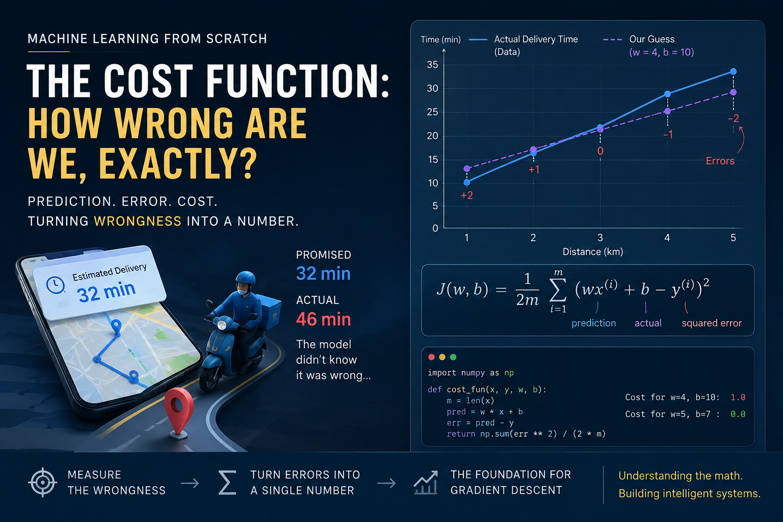
Last week, the delivery app on my phone promised my order in 32 minutes. It took 46. I wasn't really annoyed about the food being late. I was annoyed that the model behind that estimate had no way of knowing it was wrong until the food actually showed up at my door.
In the last post, we found w = 5 and b = 7 by eyeballing a clean little table, and that pair predicted delivery times almost perfectly. But that raises an obvious question: if someone else had guessed w = 4 and b = 10, how would we know which guess was better without just staring at both and going with our gut?
We need a way to turn "how wrong is this guess" into an actual number. That number has a name in machine learning. It is called the cost function. This post is about building that number from scratch, by hand first, then in code.
Here is the same delivery table from the last post.
| Distance (km) | Actual Delivery Time (min) |
|---|---|
| 1 | 12 |
| 2 | 17 |
| 3 | 22 |
| 4 | 27 |
| 5 | 32 |
We already know w = 5, b = 7 fits this table perfectly. But suppose we did not know that, and we guessed w = 4, b = 10 instead. Here is what that guess predicts for each row, and how far off it is from the actual value.
| Distance | Prediction | Actual | Error |
|---|---|---|---|
| 1 | 14 | 12 | 2 |
| 2 | 18 | 17 | 1 |
| 3 | 22 | 22 | 0 |
| 4 | 26 | 27 | −1 |
| 5 | 30 | 32 | −2 |
Now we have five errors: 2, 1, 0, −1, and −2. The question is how we combine them into one single number that tells us how good or bad this guess is overall.
The obvious first move is to just add them up: 2 + 1 + 0 + (−1) + (−2) = 0. That gives us zero, even though the predictions are clearly not perfect. The positive and negative errors simply cancel each other out.
So instead of adding the errors themselves, we square them.
2² = 4
1² = 1
0² = 0
(−1)² = 1
(−2)² = 4
Now none of the errors can cancel each other out, since squaring a negative number gives the same positive result as squaring its positive counterpart.
Squaring also makes bigger mistakes matter more. An error of 1 contributes 1, while an error of 5 contributes 25.
Add these squared errors up: 4 + 1 + 0 + 1 + 4 = 10.
We have 5 examples, so dividing by 5 gives us the mean squared error. We then include an extra factor of 1/2. That factor does not change which guess is better, but it makes the derivatives cleaner when we get to gradient descent.
cost = 10 ÷ (2 × 5) = 10 ÷ 10 = 1.0
That single number, 1.0, is the cost for the guess w = 4, b = 10.
Think of the cost as a score for a line. A perfect line gets a score of 0. Small mistakes give a small score. Large mistakes push the score up quickly. So instead of looking at five predictions and trying to judge them yourself, we have reduced the whole table to one number.
Now the cost for our original guess, w = 5 and b = 7, which we already know fits the table perfectly. Every prediction matches the actual value exactly, so every error is 0, every squared error is 0, and the total is 0 ÷ 10 = 0.
Our cost is 1.0 for the wrong guess and 0 for the right one. That number does not have a universal meaning by itself; it depends on the scale of the dataset. What matters is that, on the same dataset, a lower cost means a better fit. In this example, a cost of 1 corresponds to an RMSE of about 1.4 minutes, so the errors are relatively small compared with delivery times of 12 to 32 minutes.
We just described the cost function step by step. Now let's compress those steps into one formula.
J(w, b) = (1 / 2m) * sum of (prediction − actual) ** 2
Each piece of that formula maps directly onto something we already did by hand.
wx + b is the prediction for one example.
(wx + b) − y is the error for that example.
((wx + b) − y) ** 2 is the squared error.
The sum adds up every squared error across all m examples.
1/(2m) scales that total down, the same way dividing by 5 and then by 2 did above.
m is the number of examples we have, which is 5 in our table, and J(w, b) is the name for this whole cost. It depends on which w and b you plug in, which is why we write it as J(w, b) instead of just J. This is the standard cost function used for linear regression.
Here is a function that computes this cost, first the plain way, then the vectorized way, the same as we did with the prediction formula last time.
def cost_fun(x_list, y_list, w, b):

    m = len(x_list)
    total_err = 0

    for i in range(m):
        pred = w * x_list[i] + b
        err = pred - y_list[i]
        total_err += err ** 2

    return total_err / (2 * m)


distances = [1, 2, 3, 4, 5]
actual_times = [12, 17, 22, 27, 32]

wrong_guess = cost_fun(distances, actual_times, w=4, b=10)
correct_guess = cost_fun(distances, actual_times, w=5, b=7)

print("Cost for w=4, b=10:", wrong_guess)
print("Cost for w=5, b=7:", correct_guess)

# Cost for w=4, b=10: 1.0
# Cost for w=5, b=7: 0.0
Each line maps back to the formula directly. pred = w * x_list[i] + b is y_prediction = wx + b, the model itself. err = pred - y_list[i] is y_prediction − y, the error for that one example. total_err += err ** 2 adds up the squared errors. return total_err / (2 * m) applies the 1/(2m) scaling and gives us the cost.
That matches exactly what we worked out by hand. Now the vectorized version, using NumPy instead of a loop.
import numpy as np

def cost_fun_vectorized(x, y, w, b):
    m = len(x)
    pred = w * x + b
    err = pred - y
    return np.sum(err ** 2) / (2 * m)


distances_np = np.array([1, 2, 3, 4, 5])
actual_times_np = np.array([12, 17, 22, 27, 32])

print("Cost for w=4, b=10:", cost_fun_vectorized(distances_np, actual_times_np, w=4, b=10))
print("Cost for w=5, b=7:", cost_fun_vectorized(distances_np, actual_times_np, w=5, b=7))

# Cost for w=4, b=10: 1.0
# Cost for w=5, b=7: 0.0
There is no loop anywhere in the second version. w * x + b computes every prediction at once, pred - y computes every error at once, and np.sum(...) adds them all up in one step. The important thing is that the mathematics did not change. We only changed how we wrote the computation, and it stays fast once your dataset stops being five rows and starts being five hundred thousand.
We now have a way to measure exactly how bad a guess is. Given any w and b, we can compute a single number that tells us how well that line fits our data. We could, in theory, try a thousand different combinations of w and b, compute the cost for each one, and keep whichever combination scores lowest.
That approach falls apart quickly in practice. With one input feature you might get away with guessing enough combinations by brute force. Real models often have hundreds or thousands of these w-like numbers at once, and randomly guessing your way to the best combination of all of them would take longer than anyone could wait.
What we need instead is a way for the model to look at the cost and figure out which direction to adjust w and b in to make that cost smaller, then repeat that adjustment automatically until the cost stops improving.
We can now tell which line is worse. The harder problem is getting from a bad line to a better one without trying thousands of guesses. That is exactly where gradient descent comes in.
The full code from this post is up on GitHub here: https://github.com/tharun-pandya/Machine-Learning-Blog-Series/blob/main/Cost_Function_Of_Linear_Regression.ipynb