The Sigmoid Function: Squashing the World Into 0 and 1

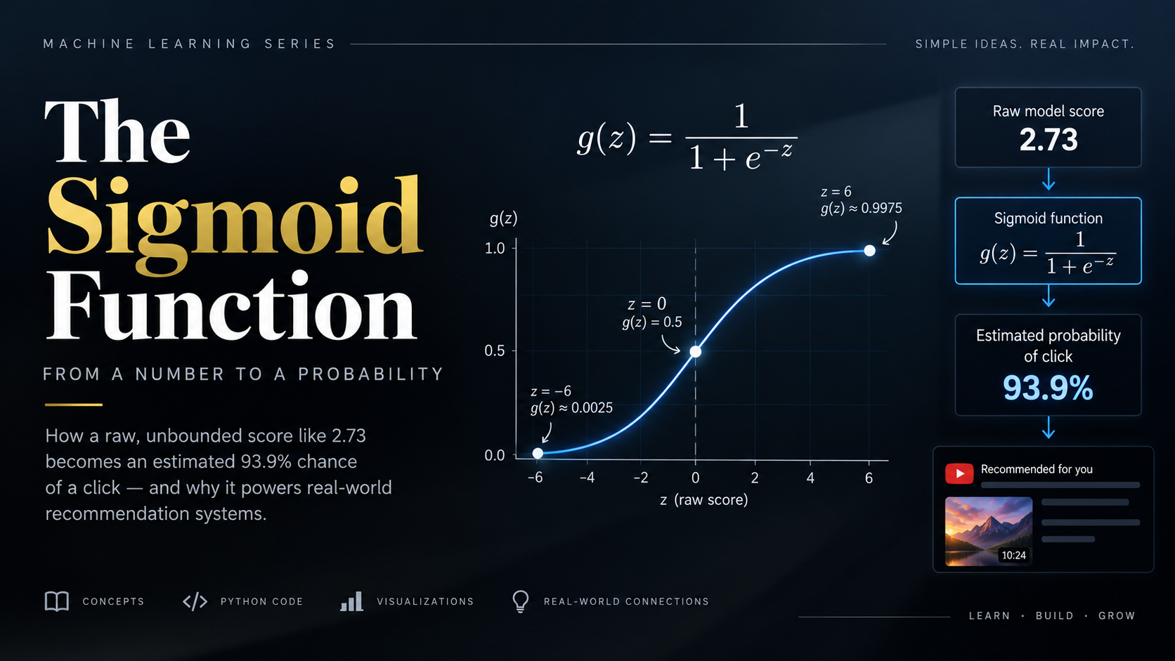
You open YouTube. You haven't searched for anything, yet the very first video looks strangely interesting. You click.

Imagine a simplified recommendation model working behind the scenes, quietly asking one question: how likely is this person to click this video? Real recommendation systems are far more complicated, but this simplified version is enough to show the idea.

Here's the catch. The raw output of a model like this usually doesn't look like a probability. It might look like this:

2.73

What does 2.73 mean? It's not 273%, because probabilities can't pass 100%. It's not 2.73% either. It's just a score, with no obvious upper limit and no obvious lower limit. It could just as easily have been -5, or 40.

So how does a raw, unbounded number like 2.73 become something like "an estimated 93.9% chance of a click"?

Picking Up Where We Left Off

This is the wall we hit at the end of the last post. We fit a straight line to a yes-or-no question, and it broke in two ways. Its predictions wandered below 0 and above 1, which makes no sense for a yes-or-no answer. And a single unusual example could drag the whole line off course.

What we need is a function that accepts any number, however large, small, or negative, and always returns something strictly between 0 and 1. That function exists, and it has a name.

Meet the Sigmoid Function

g(z) = 1 / (1 + e^(-z))

Let's unpack it. z is our raw score, the 2.73 from earlier or any number a model might produce. e is a fixed constant, roughly 2.718, that appears everywhere in math where things grow or shrink smoothly.

When I first saw e inside this formula, it looked like one more thing I was supposed to memorize. You don't need to. Treat it like pi, a constant with a fixed value, and focus on what the exponent -z is doing.

The whole trick lives in e^(-z). Let's see what it does at three values of z.

When z is very negative (say z = -6): -z becomes a large positive number, so e^(-z) becomes enormous. We're dividing 1 by "1 plus something huge," which lands very close to 0.

When z is exactly 0: e^0 is 1, always, so the formula collapses to a simple fraction:

g(0) = 1 / (1 + e^0)
     = 1 / (1 + 1)
     = 1 / 2
     = 0.5

When z is very positive (say z = 6): -z becomes a large negative number, so e^(-z) shrinks toward 0. We're dividing 1 by roughly 1 + 0, which lands very close to 1.

Here are those values, plus two in between:

z	g(z)	What it means
-6	0.0025	Very close to 0
-2	0.1192	Low
0	0.5000	Exactly in the middle
2	0.8808	High
6	0.9975	Very close to 1

Mathematically, the output is always strictly between 0 and 1. It approaches 0 as z heads toward negative infinity and approaches 1 as z heads toward positive infinity, but it never reaches either.

0 < g(z) < 1

Why the Sign of z Matters

Sigmoid doesn't only squash numbers into a range. The sign of z also tells us which side of 0.5 the output lands on:

z < 0  →  g(z) < 0.5
z = 0  →  g(z) = 0.5
z > 0  →  g(z) > 0.5

A negative score produces a probability below 0.5, a positive score produces a probability above 0.5, and a score of exactly 0 produces 0.5, where the model assigns equal estimated probability to both outcomes.

If we choose 0.5 as our classification threshold, this becomes the boundary between the two classes. That idea is the decision boundary of logistic regression, which we'll reach shortly.

Seeing the Shape

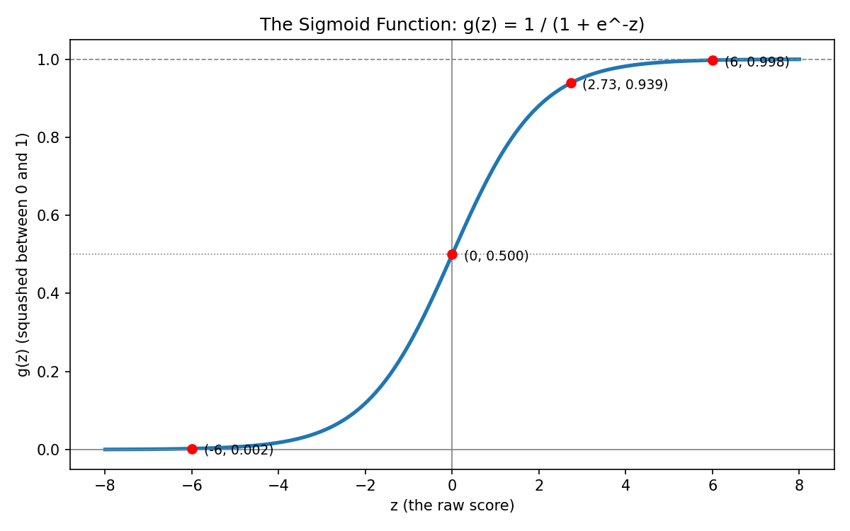
The sigmoid function maps any real-valued input to a number between 0 and 1.

This is the S-curve. It starts near 0 on the far left, rises smoothly through 0.5 in the middle, and flattens near 1 on the far right.

Notice how flat the curve is at the edges. A raw score of 6 and a raw score of 60 land in almost the same place, both extremely close to 1. However extreme a score gets, the output can never climb past 1. It runs out of room, and that's by design.

Back to Our 2.73

Now let's compute the number that opened this post.

g(2.73) = 1 / (1 + e^-2.73)

e^-2.73 works out to roughly 0.0652, so:

g(2.73) = 1 / (1 + 0.0652)
g(2.73) = 1 / 1.0652
g(2.73) = 0.9388

And 0.9388 × 100 = 93.88%, so the model's output is about 93.9%.

There's one caveat. Whether that number is a trustworthy 93.9% chance depends on the model, the data it was trained on, and how well calibrated it is. In logistic regression, we interpret g(z) as the model's estimated probability of the positive class. That's a modeling statement, not a guarantee about the real world.

Turning This Into Code

The formula translates almost directly into Python:

python

import numpy as np

def sigmoid(z):
    return 1 / (1 + np.exp(-z))

print(sigmoid(2.73))    # 0.9388
print(sigmoid(0))       # 0.5
print(sigmoid(-6))      # 0.0025, very close to 0
print(sigmoid(6))       # 0.9975, very close to 1

np.exp(-z) computes e^(-z), the same piece we worked through by hand.

To see how quickly the output saturates, print a range of values:

python

for z in [-10, -5, -2, 0, 2, 5, 10]:
    print(f"{z:>4}  ->  {sigmoid(z):.4f}")

Now plot the whole curve. This block is self-contained, so you can copy and run it as is:

python

import numpy as np
import matplotlib.pyplot as plt

def sigmoid(z):
    return 1 / (1 + np.exp(-z))

z = np.linspace(-10, 10, 200)

plt.plot(z, sigmoid(z))
plt.xlabel("z")
plt.ylabel("sigmoid(z)")
plt.title("The Sigmoid Function")
plt.grid()
plt.show()

Try changing the range of z and watch how quickly the curve flattens out. The formula, the printed numbers, and the graph are all the same function seen three ways.

A Small Hint About Training

One reason sigmoid is useful when we start training models is that its rate of change has a surprisingly simple form:

g'(z) = g(z) × (1 − g(z))

Don't worry about deriving this now. We'll derive it properly when we start optimizing models.

What We Learned

• Sigmoid takes any real number as input.

• Its output is always strictly between 0 and 1.

• z = 0 gives exactly 0.5, positive z gives more than 0.5, and negative z gives less than 0.5.

• Sigmoid can turn a model's raw score into an estimated probability.

• Sigmoid is a function, not a classifier. It doesn't predict anything by itself.

Where We Go From Here

Sigmoid doesn't know whether a student will pass an exam or whether a customer will place an order. It only sees the number we give it. That number, z, has to be produced somewhere earlier in the model, and understanding where it comes from is the next piece of the puzzle.

We already know how to combine inputs using weights and a bias. That combination can be our raw score z. Feed it into the sigmoid, and we get an estimated probability:

x₁, x₂, x₃
     ↓
w₁x₁ + w₂x₂ + w₃x₃ + b
     ↓
     z
     ↓
 sigmoid(z)
     ↓
estimated probability
     ↓
threshold (e.g. 0.5)
     ↓
prediction: yes / no

That pipeline is the basic idea behind logistic regression, and it's what the next post is about.

The full code for this post is on GitHub: github.com/tharun-pandya/Machine-Learning-Blog-Series/blob/main/sigmoid_function.ipynb

See you in the next one.