Senior AI Engineer | Building & Telling Stories about AI/ML Systems | Software Engineer
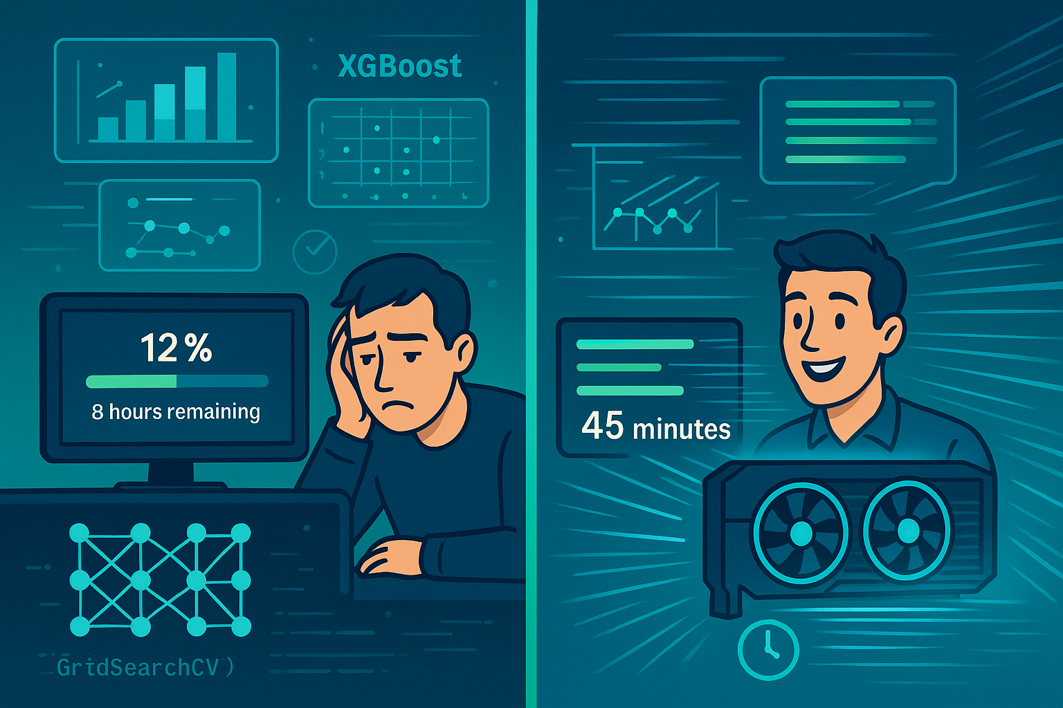
Imagine waiting 8 hours for your XGBoost hyper-parameter tuning to complete, only to discover you forgot to include a crucial parameter combination.
Sound familiar?
Every data scientist and ML/AI engineer have lived this nightmare—watching precious hours evaporate while GridSearchCV crawls through parameter combinations at a snail's pace.
The cost isn't just time; it's missed deadlines, suboptimal models, and the crushing realization that thorough hyper-parameter exploration feels impossible within project constraints.
But here's the game-changer: GPU acceleration transforms that same 8-hour search into a 45-minute sprint—with better results.
This guide reveals how combining XGBoost's GPU capabilities with GridSearchCV creates a hyperparameter tuning workflow that's not just faster, but fundamentally more effective.
You'll discover the exact setup, configuration, and optimization strategies that let you explore broader parameter spaces, iterate rapidly, and deploy superior models while your competitors are still waiting for their first search to complete.
Ready to reclaim those lost hours?
XGBoost stands as one of the most successful machine learning algorithms, dominating competitions and production environments worldwide.
However, its computational intensity becomes a bottleneck when dealing with large datasets or extensive hyperparameter searches.
Traditional CPU-based training can take hours for comprehensive parameter optimization.
GPU acceleration transforms this landscape by leveraging thousands of parallel cores to accelerate the most computationally expensive operations.
The key breakthrough lies in XGBoost's GPU histogram algorithm (gpu_hist).
Unlike traditional CPU approaches that build histograms sequentially, the GPU version constructs all feature histograms simultaneously across thousands of threads.
This parallel processing delivers 10-50x speedups for histogram building—typically the most time-consuming phase of gradient boosting. Memory optimizations ensure coalesced access patterns that maximize GPU bandwidth utilization.
Before diving into hyperparameter tuning, you need a properly configured environment. Start by installing the essential libraries with GPU support capabilities.
pip install xgboost scikit-learn pandas numpy
XGBoost automatically includes GPU support in recent PyPI wheels when CUDA is available on your system.
System-level GPU verification comes first in your setup process. Run the nvidia-smi command in your terminal to confirm GPU detection and availability.
This command displays GPU models, memory usage, driver versions, and current processes. If nvidia-smi fails or shows no devices, address GPU driver installation before continuing.
nvidia-smi
Next, verify XGBoost recognizes your GPU hardware and includes CUDA support.
Execute the following Python code to examine build information. Look specifically for "USE_CUDA": "True" in the output dictionary.
import xgboost
print(xgboost.build_info())
Learning rate
The learning rate (eta) controls the step size for updates after each boosting round.
Think of this parameter as controlling the speed of your optimization journey.
Smaller values like 0.01 create stable, methodical learning but require more iterations.
Larger values like 0.3 risk overshooting optimal solutions but train faster.
Most practitioners start with 0.1 and adjust based on convergence behavior.
Number of estimators
The number of estimators (n_estimators) determines how many boosting rounds to execute.
More trees generally improve accuracy up to a point where diminishing returns occur.
However, excessive trees lead to overfitting and longer training times.
Typical ranges span from 100 to 1000 trees, with early stopping helping find optimal points.
Max Depth
Max depth controls the complexity of individual decision trees within the ensemble.
Deeper trees capture more intricate patterns but risk memorizing training data specifics.
Shallow trees around depth 3-4 work well for simpler datasets. Complex datasets might benefit from depths up to 8-10 trees. Balance complexity needs against overfitting risks when selecting ranges.
Minimum child weight
Minimum child weight sets the threshold for creating new leaf nodes. Higher values prevent splits affecting only a few samples, reducing overfitting.
This parameter acts as a regularization mechanism for tree growth. Values typically range from 1 to 10, with higher values creating more conservative models. Adjust based on dataset size and noise levels.
Subsample
Subsample determines the fraction of training data used for each tree.
Values less than 1.0 introduce randomness that helps prevent overfitting. This stochastic approach improves generalization by ensuring diverse tree perspectives.
Common values range from 0.7 to 1.0, with lower values providing stronger regularization. Balance randomness benefits against information loss when selecting values.
Column sampling
Column sampling (colsample_bytree) controls feature randomness per tree.
This parameter forces the model to explore different feature combinations. Feature randomness creates more robust models less dependent on specific predictors.
Values typically range from 0.6 to 1.0 based on dataset characteristics. High-dimensional datasets often benefit from more aggressive feature sampling.
Single GPU configuration provides the foundation for most hyperparameter tuning scenarios.
The gpu_hist tree method activates GPU-accelerated histogram algorithms.
GPU ID specification becomes crucial in multi-GPU systems for device selection.
The GPU predictor ensures both training and inference utilize GPU acceleration.
gpu_params = {
    'tree_method': 'gpu_hist',
    'gpu_id': 0,
    'predictor': 'gpu_predictor'
}
Multi-GPU setups require additional parameter considerations for optimal performance.
Modern XGBoost versions recommend using Dask for distributed multi-GPU training.
The n_gpus parameter historically controlled GPU utilization but faces deprecation.
multi_gpu_params = {
    'tree_method': 'gpu_hist',
    'n_gpus': -1,  # Use all available GPUs (deprecated)
    'predictor': 'gpu_predictor'
}
Manual hyper-parameter exploration provides intuition before systematic searches.
Start with single parameter variations to understand individual impacts.
Cross-validation ensures robust performance estimates across different data splits.
This approach helps identify promising parameter ranges for comprehensive searches.
import numpy as np
import xgboost as xgb
from sklearn.model_selection import StratifiedKFold
from sklearn.metrics import roc_auc_score

def evaluate_max_depth(X, y, max_depths=[3, 5, 7, 10]):
    results = {}

    for depth in max_depths:
        print(f"Evaluating max_depth = {depth}")
        skf = StratifiedKFold(n_splits=3, shuffle=True, random_state=42)
        scores = []

        for train_idx, val_idx in skf.split(X, y):
            model = xgb.XGBClassifier(
                max_depth=depth,
                tree_method="gpu_hist",
                predictor="gpu_predictor",
                use_label_encoder=False,
                eval_metric="auc"
            )

            model.fit(X[train_idx], y[train_idx])
            preds = model.predict_proba(X[val_idx])[:, 1]
            scores.append(roc_auc_score(y[val_idx], preds))

        avg_score = np.mean(scores)
        std_score = np.std(scores)
        results[depth] = {'mean': avg_score, 'std': std_score}

        print(f"Max depth {depth}: {avg_score:.4f} ± {std_score:.4f}")

    return results
Parameter grid definition requires balancing exploration breadth with computational feasibility.
Start with coarse grids covering wide parameter ranges to identify promising regions.
Refine grids around high-performing areas for detailed optimization.
Consider parameter interactions when defining multidimensional search spaces.
from sklearn.model_selection import GridSearchCV

# Comprehensive parameter grid
param_grid = {
    'max_depth': [3, 5, 7, 9],
    'learning_rate': [0.01, 0.05, 0.1, 0.2],
    'n_estimators': [100, 200, 400, 800],
    'subsample': [0.7, 0.8, 0.9, 1.0],
    'colsample_bytree': [0.7, 0.8, 0.9, 1.0],
    'min_child_weight': [1, 3, 5, 7],
    'gamma': [0, 0.1, 0.5, 1.0]
}
GridSearchCV configuration balances thoroughness with computational efficiency.
Set n_jobs to 1 when using GPU acceleration to avoid thread conflicts.
Choose appropriate scoring metrics that align with your problem objectives.
Verbose output helps monitor progress during lengthy parameter searches.
# Initialize XGBoost with GPU parameters
xgb_clf = xgb.XGBClassifier(
    objective='binary:logistic',
    tree_method='gpu_hist',
    predictor='gpu_predictor',
    use_label_encoder=False,
    eval_metric='auc'
)

# Configure GridSearchCV
grid_search = GridSearchCV(
    estimator=xgb_clf,
    param_grid=param_grid,
    scoring='roc_auc',
    cv=3,
    verbose=2,
    n_jobs=1,  # Essential for GPU training
    return_train_score=False
)

# Execute parameter search
grid_search.fit(X_train, y_train)
Comprehensive results analysis goes beyond identifying the best parameters.
Examine the distribution of scores across parameter combinations.
Look for patterns indicating parameter sensitivity and interaction effects.
Validate best parameters on independent test sets to confirm generalization.
# Extract best results
best_params = grid_search.best_params_
best_score = grid_search.best_score_
best_model = grid_search.best_estimator_

print(f"Best parameters: {best_params}")
print(f"Best cross-validation AUC: {best_score:.4f}")

# Test set validation
test_predictions = best_model.predict_proba(X_test)[:, 1]
test_auc = roc_auc_score(y_test, test_predictions)
print(f"Test set AUC: {test_auc:.4f}")
Dataset characteristics heavily influence optimal hyperparameter ranges.
Large datasets benefit from more conservative regularization to prevent overfitting.
Small datasets require aggressive regularization and simpler models.
High-dimensional data needs feature sampling to improve generalization.
Feature engineering quality impacts hyper-parameter sensitivity significantly. Well-engineered features reduce model complexity requirements.
Raw features might need deeper trees and stronger regularization. Consider feature selection before extensive hyper-parameter tuning.
Production environments impose additional constraints on model selection.
Inference speed requirements might favor shallower trees despite accuracy costs.
Memory constraints limit model complexity in resource-constrained environments.
Model interpretability needs might influence tree depth and feature usage decisions.
Model performance monitoring ensures continued effectiveness in production.
Track key metrics like accuracy, inference speed, and resource utilization.
Schedule periodic retraining with updated hyper-parameter searches.
Monitor for data drift that might require parameter adjustments.
GPU-accelerated XGBoost hyper-parameter tuning with GridSearchCV transforms machine learning workflows from time-consuming manual processes into efficient, systematic optimization procedures.
The combination of parallel GPU processing, comprehensive parameter exploration, and robust cross-validation delivers superior models in dramatically reduced timeframes.
This approach enables practitioners to explore broader parameter spaces, iterate faster, and ultimately deploy better-performing models.
The key to success lies in understanding the interplay between XGBoost parameters, GPU optimization techniques, and systematic search strategies.
Start with proper environment setup and GPU verification before progressing to comprehensive parameter searches.
Balance exploration breadth with computational constraints through hierarchical search approaches.
Always validate results on independent test sets to ensure robust generalization performance.
Future developments in GPU-accelerated machine learning promise even greater performance improvements.
Multi-GPU distributed training will enable handling of massive datasets and parameter spaces.
Automated machine learning techniques will further streamline the hyper-parameter optimization process.
Integration with cloud computing platforms will democratize access to high-performance GPU resources for machine learning practitioners worldwide.
PS:
If you like this article, share it with others ♻️
Would help a lot ❤️
And feel free to follow me for more content like this.