保留正文与补采附件。源页面当前未重新核验;具体限制见交付清单。
 We value your privacy
We use cookies to enhance your browsing experience, serve personalised ads or content, and analyse our traffic. By clicking "Accept All", you consent to our use of cookies.
Customise Reject All Accept All
Customise Consent Preferences
 We use cookies to help you navigate efficiently and perform certain functions. You will find detailed information about all cookies under each consent category below.
The cookies that are categorised as "Necessary" are stored on your browser as they are essential for enabling the basic functionalities of the site. ... Show more
NecessaryAlways Active
Necessary cookies are required to enable the basic features of this site, such as providing secure log-in or adjusting your consent preferences. These cookies do not store any personally identifiable data.
-
Cookie
BCTempID
-
Duration
10 minutes
-
Description
No description available.
-
Cookie
__cf_bm
-
Duration
1 hour
-
Description
This cookie, set by Cloudflare, is used to support Cloudflare Bot Management.
-
Cookie
AWSALBCORS
-
Duration
7 days
-
Description
Amazon Web Services set this cookie for load balancing.
-
Cookie
_cfuvid
-
Duration
session
-
Description
Cloudflare sets this cookie to track users across sessions to optimize user experience by maintaining session consistency and providing personalized services
-
Cookie
li_gc
-
Duration
6 months
-
Description
Linkedin set this cookie for storing visitor's consent regarding using cookies for non-essential purposes.
-
Cookie
__hssrc
-
Duration
session
-
Description
This cookie is set by Hubspot whenever it changes the session cookie. The __hssrc cookie set to 1 indicates that the user has restarted the browser, and if the cookie does not exist, it is assumed to be a new session.
-
Cookie
__hssc
-
Duration
1 hour
-
Description
HubSpot sets this cookie to keep track of sessions and to determine if HubSpot should increment the session number and timestamps in the __hstc cookie.
-
Cookie
wpEmojiSettingsSupports
-
Duration
session
-
Description
WordPress sets this cookie when a user interacts with emojis on a WordPress site. It helps determine if the user's browser can display emojis properly.
-
Cookie
BCSessionID
-
Duration
1 year 1 month 4 days
-
Description
Blueconic sets this cookie as a unique identifier for the BlueConic profile.
-
Cookie
_octo
-
Duration
1 year
-
Description
No description available.
-
Cookie
logged_in
-
Duration
1 year
-
Description
No description available.
-
Cookie
__Secure-YEC
-
Duration
past
-
Description
YouTube sets this cookie to stores the user's video player preferences using embedded YouTube video
-
Cookie
__eoi
-
Duration
6 months
-
Description
Description is currently not available.
-
Cookie
AWSALBTGCORS
-
Duration
7 days
-
Description
No description available.
-
Cookie
login-status-p
-
Duration
past
-
Description
Description is currently not available.
-
Cookie
AWSALBTG
-
Duration
7 days
-
Description
No description available.
-
Cookie
csrf_token
-
Duration
session
-
Description
No description available.
-
Cookie
token_v2
-
Duration
1 day
-
Description
Description is currently not available.
-
Cookie
D
-
Duration
1 year
-
Description
Description is currently not available.
-
Cookie
PHPSESSID
-
Duration
session
-
Description
This cookie is native to PHP applications. The cookie stores and identifies a user's unique session ID to manage user sessions on the website. The cookie is a session cookie and will be deleted when all the browser windows are closed.
-
Cookie
VISITOR_PRIVACY_METADATA
-
Duration
6 months
-
Description
YouTube sets this cookie to store the user's cookie consent state for the current domain.
-
Cookie
cookietest
-
Duration
session
-
Description
The cookietest cookie is typically used to determine whether the user's browser accepts cookies, essential for website functionality and user experience.
-
Cookie
__Host-airtable-session
-
Duration
1 year
-
Description
This cookie is used to enable us to integrate the services of Airtable.
-
Cookie
__Host-airtable-session.sig
-
Duration
1 year
-
Description
This cookie is used to enable us to integrate the services of Airtable.
-
Cookie
m
-
Duration
1 year 1 month 4 days
-
Description
Stripe sets this cookie for fraud prevention purposes. It identifies the device used to access the website, allowing the website to be formatted accordingly.
-
Cookie
BIGipServer*
-
Duration
session
-
Description
Marketo sets this cookie to collect information about the user's online activity and build a profile about their interests to provide advertisements relevant to the user.
-
Cookie
__cfruid
-
Duration
session
-
Description
Cloudflare sets this cookie to identify trusted web traffic.
-
Cookie
_GRECAPTCHA
-
Duration
6 months
-
Description
Google Recaptcha service sets this cookie to identify bots to protect the website against malicious spam attacks.
-
Cookie
__Secure-YNID
-
Duration
6 months
-
Description
Google cookie used to protect user security and prevent fraud, especially during the login process.
-
Cookie
cookieyes-consent
-
Duration
1 year
-
Description
CookieYes sets this cookie to remember users' consent preferences so that their preferences are respected on subsequent visits to this site. It does not collect or store any personal information about the site visitors.
Functional
Functional cookies help perform certain functionalities like sharing the content of the website on social media platforms, collecting feedback, and other third-party features.
-
Cookie
lidc
-
Duration
1 day
-
Description
LinkedIn sets the lidc cookie to facilitate data center selection.
-
Cookie
brw
-
Duration
1 year
-
Description
No description available.
-
Cookie
brwConsent
-
Duration
5 minutes
-
Description
Description is currently not available.
-
Cookie
WMF-Uniq
-
Duration
1 year
-
Description
Description is currently not available.
-
Cookie
loom_anon_comment
-
Duration
1 year
-
Description
No description available.
-
Cookie
loom_referral_video
-
Duration
session
-
Description
Description is currently not available.
-
Cookie
VISITOR_INFO1_LIVE
-
Duration
6 months
-
Description
A cookie set by YouTube to measure bandwidth that determines whether the user gets the new or old player interface.
-
Cookie
yt-remote-connected-devices
-
Duration
Never Expires
-
Description
YouTube sets this cookie to store the user's video preferences using embedded YouTube videos.
-
Cookie
ytidb::LAST_RESULT_ENTRY_KEY
-
Duration
Never Expires
-
Description
The cookie ytidb::LAST_RESULT_ENTRY_KEY is used by YouTube to store the last search result entry that was clicked by the user. This information is used to improve the user experience by providing more relevant search results in the future.
-
Cookie
yt-remote-device-id
-
Duration
Never Expires
-
Description
YouTube sets this cookie to store the user's video preferences using embedded YouTube videos.
-
Cookie
yt-remote-session-name
-
Duration
session
-
Description
The yt-remote-session-name cookie is used by YouTube to store the user's video player preferences using embedded YouTube video.
-
Cookie
yt-remote-fast-check-period
-
Duration
session
-
Description
The yt-remote-fast-check-period cookie is used by YouTube to store the user's video player preferences for embedded YouTube videos.
-
Cookie
yt-remote-session-app
-
Duration
session
-
Description
The yt-remote-session-app cookie is used by YouTube to store user preferences and information about the interface of the embedded YouTube video player.
-
Cookie
yt-remote-cast-available
-
Duration
session
-
Description
The yt-remote-cast-available cookie is used to store the user's preferences regarding whether casting is available on their YouTube video player.
-
Cookie
yt-remote-cast-installed
-
Duration
session
-
Description
The yt-remote-cast-installed cookie is used to store the user's video player preferences using embedded YouTube video.
-
Cookie
cp_session
-
Duration
3 months
-
Description
Codepen sets this cookie for Help systems found in the website.
-
Cookie
loid
-
Duration
1 year 1 month 4 days
-
Description
This cookie is set by the Reddit. The cookie enables the sharing of content from the website onto the social media platform.
Analytics
Analytical cookies are used to understand how visitors interact with the website. These cookies help provide information on metrics such as the number of visitors, bounce rate, traffic source, etc.
-
Cookie
__hstc
-
Duration
6 months
-
Description
Hubspot set this main cookie for tracking visitors. It contains the domain, initial timestamp (first visit), last timestamp (last visit), current timestamp (this visit), and session number (increments for each subsequent session).
-
Cookie
hubspotutk
-
Duration
6 months
-
Description
HubSpot sets this cookie to keep track of the visitors to the website. This cookie is passed to HubSpot on form submission and used when deduplicating contacts.
-
Cookie
_ga
-
Duration
1 year 1 month 4 days
-
Description
Google Analytics sets this cookie to calculate visitor, session and campaign data and track site usage for the site's analytics report. The cookie stores information anonymously and assigns a randomly generated number to recognise unique visitors.
-
Cookie
ga*
-
Duration
1 year 1 month 4 days
-
Description
Google Analytics sets this cookie to store and count page views.
-
Cookie
__Host-psifi.analyticsTrace
-
Duration
6 hours
-
Description
Description is currently not available.
-
Cookie
__Host-psifi.analyticsTraceV2
-
Duration
6 hours
-
Description
Description is currently not available.
-
Cookie
_gh_sess
-
Duration
session
-
Description
GitHub sets this cookie for temporary application and framework state between pages like what step the user is on in a multiple step form.
-
Cookie
YSC
-
Duration
session
-
Description
YSC cookie is set by Youtube and is used to track the views of embedded videos on Youtube pages.
-
Cookie
ajs_anonymous_id
-
Duration
1 year
-
Description
This cookie is set by Segment to count the number of people who visit a certain site by tracking if they have visited before.
-
Cookie
vuid
-
Duration
1 year 1 month 4 days
-
Description
Vimeo installs this cookie to collect tracking information by setting a unique ID to embed videos on the website.
Performance
Performance cookies are used to understand and analyse the key performance indexes of the website which helps in delivering a better user experience for the visitors.
-
Cookie
AWSALB
-
Duration
7 days
-
Description
AWSALB is an application load balancer cookie set by Amazon Web Services to map the session to the target.
-
Cookie
acq
-
Duration
past
-
Description
Description is currently not available.
-
Cookie
acq.sig
-
Duration
past
-
Description
Description is currently not available.
-
Cookie
ptc
-
Duration
2 years
-
Description
No description available.
Advertisement
Advertisement cookies are used to provide visitors with customised advertisements based on the pages you visited previously and to analyse the effectiveness of the ad campaigns.
-
Cookie
muc_ads
-
Duration
1 year 1 month 4 days
-
Description
Twitter sets this cookie to collect user behaviour and interaction data to optimize the website.
-
Cookie
guest_id_marketing
-
Duration
1 year 1 month 4 days
-
Description
Twitter sets this cookie to identify and track the website visitor.
-
Cookie
guest_id_ads
-
Duration
1 year 1 month 4 days
-
Description
Twitter sets this cookie to identify and track the website visitor.
-
Cookie
personalization_id
-
Duration
1 year 1 month 4 days
-
Description
Twitter sets this cookie to integrate and share features for social media and also store information about how the user uses the website, for tracking and targeting.
-
Cookie
guest_id
-
Duration
1 year 1 month 4 days
-
Description
Twitter sets this cookie to identify and track the website visitor. It registers if a user is signed in to the Twitter platform and collects information about ad preferences.
-
Cookie
bcookie
-
Duration
1 year
-
Description
LinkedIn sets this cookie from LinkedIn share buttons and ad tags to recognize browser IDs.
-
Cookie
__Secure-ROLLOUT_TOKEN
-
Duration
6 months
-
Description
YouTube sets this cookie to manage feature rollout and experimentation. It helps Google control which new features or interface changes are shown to users as part of testing and staged rollouts, ensuring consistent experience for a given user during an experiment.
-
Cookie
yt.innertube::nextId
-
Duration
Never Expires
-
Description
YouTube sets this cookie to register a unique ID to store data on what videos from YouTube the user has seen.
-
Cookie
yt.innertube::requests
-
Duration
Never Expires
-
Description
YouTube sets this cookie to register a unique ID to store data on what videos from YouTube the user has seen.
-
Cookie
session_tracker
-
Duration
session
-
Description
This cookie is set by the Reddit. This cookie is used to identify trusted web traffic. It also helps in adverstising on the website.
-
Cookie
edgebucket
-
Duration
session
-
Description
Reddit sets this cookie to save the information about a log-on Reddit user, for the purpose of advertisement recommendations and updating the content.
-
Cookie
did
-
Duration
1 year
-
Description
Arbor sets this cookie to show targeted ads to site visitors.This cookie expires after 2 months or 1 year.
Uncategorised
Other uncategorised cookies are those that are being analysed and have not been classified into a category as yet.
No cookies to display.
Reject All Save My Preferences Accept All
Toggle SearchToggle Mobile Navigation
Publish AI, ML & data-science insights to a global community of data professionals.
Sign inSubmit an Article
LatestEditor's PicksNewsletterShipAI
Write For TDS
LinkedInXToggle Search
Artificial Intelligence
Pearson vs Spearman Correlation: Find Harmony between the Variables
Which measure of correlation should you use for your task? Learn all you need to know about Pearson and Spearman correlations.
Riccardo Andreoni
January 18, 20246 min read
Which measure of correlation should you use for your task? Learn all you need to know about Pearson and Spearman correlations
Consider a symphony orchestra tuning their instruments before a performance. Each musician adjusts their notes to harmonize with others, ensuring a seamless musical experience. In Data Science , the variables in a dataset can be compared to the orchestra's musicians : understanding the harmony or dissonances between them is crucial.
 Image source: pixabay.com.
Correlation is a statistical measure that acts like the conductor of the orchestra, guiding the understanding of the complex relationships within our data. Here we will focus on two types of correlations: Pearson and Spearman.
If our data is a composition, Pearson and Spearman are our orchestra's conductors : they have a singular style of interpreting the symphony, each with peculiar strengths and subtleties. Understanding these two different methodologies will allow you to extract insights and understand the connections between variables.
Learn this step by step with the interactive AI Engineer, AI and Data Scientist, Computer Science, Data Analyst and Machine Learning roadmaps.
Pearson Correlation
The Pearson correlation coefficient , denoted as r , quantifies the strength and direction of a linear relationship between two continuous variables [1]. It is calculated by dividing the covariance of the two variables by the product of their standard deviations.
 Pearson coefficient formula
Here X and Y are two different variables, and _X i and _Y i represent individual data points. bar{X} and bar{Y} denote the mean values of the respective variables.
The interpretation of r relies on its value, ranging from -1 to 1. A value of -1 implies a perfect negative correlation, indicating that as one variable increases, the other decreases linearly [2]. Conversely, a value of 1 signifies a perfect positive correlation, illustrating a linear increase in both variables. A value of 0 implies no linear correlation.
Pearson correlation is particularly good at capturing linear relationships between variables. Its sensitivity to linear patterns makes it a powerful tool when investigating relationships governed by a consistent linear trend. Moreover, the standardized nature of the coefficient allows for easy comparison across different datasets.
However, it's crucial to note that Pearson is susceptible to the influence of outliers. If a dataset contains extreme values they can impact the calculation, leading to inaccurate interpretations.
Technical concepts can be better understood through practical examples. Let's use Python to show the computation of Pearson correlation and its visualization. Suppose we have two lists representing the hours spent studying (X) and the corresponding exam scores (Y).
python
import numpy as np
from scipy.stats import pearsonr
import matplotlib.pyplot as plt
import seaborn as sns

# Generating data points
np.random.seed(42)  # For reproducibility
hours_studied = np.random.randint(8, 25, size=50)
exam_scores = 60 + 2 * hours_studied + np.random.normal(0, 5, size=50)

# Calculate Pearson correlation coefficient
pearson_corr, _ = pearsonr(hours_studied, exam_scores)

# Calculate Pearson correlation line coefficients
m, b = np.polyfit(hours_studied, exam_scores, 1)  # Fit a linear regression line

# Scatter plot
fig, ax = plt.subplots()
ax.scatter(hours_studied, exam_scores, color=sns.color_palette("hls",24)[14], alpha=.9, label='Data points')
plt.plot(hours_studied, m * np.array(hours_studied) + b, color='red', alpha=.6, label='Pearson Correlation Line')
plt.title("Hours Studied vs. Exam Scores")
plt.xlabel("Hours Studied")
plt.ylabel("Exam Scores")
plt.legend(loc='lower right')
ax.spines['top'].set_visible(False)
ax.spines['bottom'].set_visible(False)
ax.spines['right'].set_visible(False)
ax.spines['left'].set_visible(False)
ax.xaxis.set_ticks_position('none')
ax.yaxis.set_ticks_position('none')
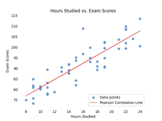 Image by the author.
 Pearson correlation effectiveness diminishes when faced with curvilinear patterns. This limitation arises from Pearson's inherent assumption of linearity, making it ill-suited to capture the nuances of non-linear relationships.
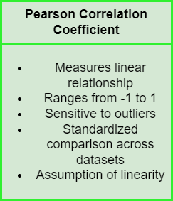 Image by the author.
Consider a scenario where the relationship between two variables follows a quadratic curve. Pearson correlation might inaccurately suggest a weak or nonexistent relationship due to its inability to capture the non-linear relation.
python
# Generating quadratic data
np.random.seed(42)
X = np.linspace(-10, 10, 100)
Y = X**2 + np.random.normal(0, 10, size=len(X))

# Calculate Pearson correlation coefficient
pearson_corr, _ = pearsonr(X, Y)

m, b = np.polyfit(X, Y, 1)  # Fit a linear regression line

# Scatter plot
fig, ax = plt.subplots()
ax.scatter(X, Y, color=sns.color_palette("hls",24)[14], alpha=.9, label='Data points')
plt.plot(X, m * X + b, color='red', alpha=.6, label='Pearson Correlation Line')
plt.title("X vs. Y (Quadratic Relationship)")
plt.xlabel("X")
plt.ylabel("Y")
plt.legend(loc='upper center')
ax.spines['top'].set_visible(False)
ax.spines['bottom'].set_visible(False)
ax.spines['right'].set_visible(False)
ax.spines['left'].set_visible(False)
ax.xaxis.set_ticks_position('none')
ax.yaxis.set_ticks_position('none')

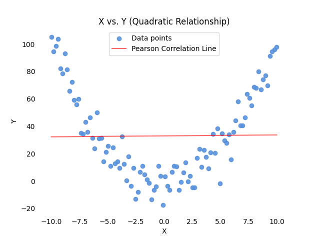 Image by the author.
Spearman Correlation
Spearman correlation addresses the limitations of Pearson when applied to non-linear relationships or datasets containing outliers [3]. Spearman's rank correlation coefficient (ρ), denoted as rho , operates on the ranked values of variables, making it less sensitive to extreme values and well-suited for capturing monotonic relationships.
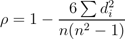 Spearman coefficient formula
In the above formula, _d i represents the difference between the ranks of corresponding pairs of variables, and n is the number of data points.
Similar to Pearson, Spearman's coefficient ranges from -1 to 1. A value of -1 indicates a perfect negative monotonic correlation, meaning that as one variable increases, the other consistently decreases. A value of 1 signifies a perfect positive monotonic correlation, illustrating a consistent increase in both variables. A value of 0 denotes no monotonic correlation.
Unlike Pearson, Spearman does not assume linearity and is robust in case of outliers. It focuses on the ordinal nature of data, making it a valuable tool when the relationship between variables is more about the order than the specific values.
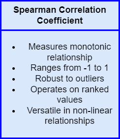 Image by the author.
Consider the following practical application using Python, where we have two variables 'A' and 'B' with a non-linear relationship:
python
import numpy as np
from scipy.stats import spearmanr
from scipy.stats import pearsonr
import matplotlib.pyplot as plt

# Generating non-linear data
np.random.seed(42)
A = np.linspace(-10, 10, 100)
B = A**5 + np.random.normal(0, 4000, size=len(A))

# Calculate Spearman correlation coefficient
spearman_corr, _ = spearmanr(A, B)
# Calculate Pearson correlation coefficient
pearson_corr, _ = pearsonr(A, B)
m, b = np.polyfit(A, B, 1)  # Fit a linear regression line

# Scatter plot
fig, ax = plt.subplots()
ax.scatter(A, B, color=sns.color_palette("hls",24)[14], alpha=.9, label='Data points')
plt.plot(X, m * X + b, color='red', alpha=.6, label='Pearson Correlation Line')
plt.title("A vs. B (Non-linear Relationship)")
plt.xlabel("A")
plt.ylabel("B")
ax.spines['top'].set_visible(False)
ax.spines['bottom'].set_visible(False)
ax.spines['right'].set_visible(False)
ax.spines['left'].set_visible(False)
ax.xaxis.set_ticks_position('none')
ax.yaxis.set_ticks_position('none')

plt.legend()
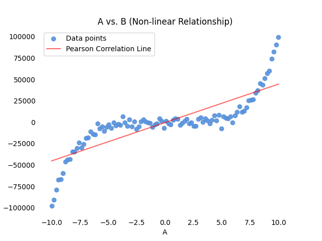 Image by the author.
In this example, the scatter plot visualizes a non-linear relationship between variables 'A' and 'B.' Spearman correlation, which does not assume linearity, will be better suited to capture and quantify this non-linear association. You can see that the red line, representing the Pearson Correlation Line, misses the nature of the variables' relationship.
We can quantify this measure by comparing the two coefficients:
 Spearman coefficient is sensibly higher, as it is more suited for this type of relationship.
Conclusion: Pearson vs. Spearman
Concluding this introductory guide, let's point out the pros and cons of the two measures.
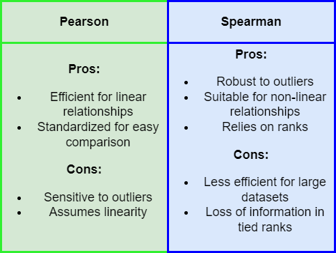 Image by the author.
Pearson Correlation coefficient is indeed efficient for linear relationship , and can provide a standardized measure for easy comparison across different datasets.
On the other hand, Pearson coefficient is highly sensitive to outliers. Also, assuming linearity may mislead in non-linear scenarios.
Most of Pearson coefficient's downsides are addressed by Spearman Correlation coefficient: it is robust in the presence of outliers , and, as it relies on the rank of data points , it is suitable for non-linear relationships.
It is important, however, to keep in mind that Spearman coefficient has also some criticalities. In my opinion the most relevant ones are its lower efficiency on large datasets, and the potential loss of information in case of tied ranks.
In order to keep this guide concise and practical , my advice is to choose Pearson for linear relationships in normally distributed data without outliers. Opt for Spearman when facing non-linear relationships, ordinal data, or datasets with outliers, as it excels in capturing monotonic associations.
Remember that this choice heavily relies on the characteristics of the data. Keep also in mind that this introduction, while touching most important aspects, merely scratched the surface of statistical methodologies. For further study, you can find an interesting set of resources below!
References
In-text references:
[1] Laerd Statistics - Pearson Product-Moment Correlation
[2] Boston University - Correlation and Regression with R
[3] Analytics Vidhya - Pearson vs Spearman Correlation Coefficients
[4] Statistics by Jim - Spearman's Correlation Explained
Other material:
Register Now to Continue Reading
Unlock Towards Data Science with a Free Account
All articles on Towards Data Science are available to registered users. Create a free account today to access this article and thousands more.
Register for freeSign in to your account
 Written By
See all from Riccardo Andreoni
Artificial IntelligenceData ScienceMachine LearningProgrammingStatistics
Share This Article
Towards Data Science is a community publication. Submit your insights to reach our global audience and earn through the TDS Author Payment Program.
Write for TDS
Related Articles
Programming
A study of the linear congruential generator and its weaknesses
Ayoub Omari
September 9, 20229 min read
Deep Learning
Build a merchant names cleaning engine with a pre-trained spaCy deep learning model...
Cheng
January 31, 202114 min read
Machine Learning
On the importance of understanding and disregarding technical considerations in applied machine learning.
Noah Burbank
June 9, 202116 min read
Data Science
A skills framework establishes common ground for conversations, even among people of wildly diverging perspectives.
Schaun Wheeler
February 27, 201817 min read
Artificial Intelligence
This is how Surrogate Modelling is revolutionizing the world of Aerospace Engineering, from theory to practice
Piero Paialunga
August 15, 202410 min read
Artificial Intelligence
The easiest way to create a simple AI chatbot for beginners
Anass El Houd
August 19, 20205 min read
Artificial Intelligence
A Step by Step walk through of my improved Used Car Price Predictor
Terence Shin, MSc, MBA
January 15, 20208 min read
Machine Learning
How to increase the size of your dataset for later use on NLP classification tasks....
Claudio Mazzoni
May 21, 20219 min read
Programming
An overview of different Rust's built-in data structures and a deep dive into the Ndarray library
Mahmoud Harmouch
May 2, 202334 min read
Your home for data science and AI. The world's leading publication for data science, data analytics, data engineering, machine learning, and artificial intelligence professionals.
Subscribe to Our NewsletterWrite For TDS•About•Advertise•Privacy Policy•Terms of Use
© Insight Media Group, LLC 2026•The New Stack•roadmap.sh•Creator Network
Recommended Articles
Close