保留正文与补采附件。源页面当前未重新核验;具体限制见交付清单。
 We value your privacy
We use cookies to enhance your browsing experience, serve personalised ads or content, and analyse our traffic. By clicking "Accept All", you consent to our use of cookies.
Customise Reject All Accept All
Customise Consent Preferences
 We use cookies to help you navigate efficiently and perform certain functions. You will find detailed information about all cookies under each consent category below.
The cookies that are categorised as "Necessary" are stored on your browser as they are essential for enabling the basic functionalities of the site. ... Show more
NecessaryAlways Active
Necessary cookies are required to enable the basic features of this site, such as providing secure log-in or adjusting your consent preferences. These cookies do not store any personally identifiable data.
-
Cookie
BCTempID
-
Duration
10 minutes
-
Description
No description available.
-
Cookie
__cf_bm
-
Duration
1 hour
-
Description
This cookie, set by Cloudflare, is used to support Cloudflare Bot Management.
-
Cookie
AWSALBCORS
-
Duration
7 days
-
Description
Amazon Web Services set this cookie for load balancing.
-
Cookie
_cfuvid
-
Duration
session
-
Description
Cloudflare sets this cookie to track users across sessions to optimize user experience by maintaining session consistency and providing personalized services
-
Cookie
li_gc
-
Duration
6 months
-
Description
Linkedin set this cookie for storing visitor's consent regarding using cookies for non-essential purposes.
-
Cookie
__hssrc
-
Duration
session
-
Description
This cookie is set by Hubspot whenever it changes the session cookie. The __hssrc cookie set to 1 indicates that the user has restarted the browser, and if the cookie does not exist, it is assumed to be a new session.
-
Cookie
__hssc
-
Duration
1 hour
-
Description
HubSpot sets this cookie to keep track of sessions and to determine if HubSpot should increment the session number and timestamps in the __hstc cookie.
-
Cookie
wpEmojiSettingsSupports
-
Duration
session
-
Description
WordPress sets this cookie when a user interacts with emojis on a WordPress site. It helps determine if the user's browser can display emojis properly.
-
Cookie
BCSessionID
-
Duration
1 year 1 month 4 days
-
Description
Blueconic sets this cookie as a unique identifier for the BlueConic profile.
-
Cookie
_octo
-
Duration
1 year
-
Description
No description available.
-
Cookie
logged_in
-
Duration
1 year
-
Description
No description available.
-
Cookie
__Secure-YEC
-
Duration
past
-
Description
YouTube sets this cookie to stores the user's video player preferences using embedded YouTube video
-
Cookie
__eoi
-
Duration
6 months
-
Description
Description is currently not available.
-
Cookie
AWSALBTGCORS
-
Duration
7 days
-
Description
No description available.
-
Cookie
login-status-p
-
Duration
past
-
Description
Description is currently not available.
-
Cookie
AWSALBTG
-
Duration
7 days
-
Description
No description available.
-
Cookie
csrf_token
-
Duration
session
-
Description
No description available.
-
Cookie
token_v2
-
Duration
1 day
-
Description
Description is currently not available.
-
Cookie
D
-
Duration
1 year
-
Description
Description is currently not available.
-
Cookie
PHPSESSID
-
Duration
session
-
Description
This cookie is native to PHP applications. The cookie stores and identifies a user's unique session ID to manage user sessions on the website. The cookie is a session cookie and will be deleted when all the browser windows are closed.
-
Cookie
VISITOR_PRIVACY_METADATA
-
Duration
6 months
-
Description
YouTube sets this cookie to store the user's cookie consent state for the current domain.
-
Cookie
cookietest
-
Duration
session
-
Description
The cookietest cookie is typically used to determine whether the user's browser accepts cookies, essential for website functionality and user experience.
-
Cookie
__Host-airtable-session
-
Duration
1 year
-
Description
This cookie is used to enable us to integrate the services of Airtable.
-
Cookie
__Host-airtable-session.sig
-
Duration
1 year
-
Description
This cookie is used to enable us to integrate the services of Airtable.
-
Cookie
m
-
Duration
1 year 1 month 4 days
-
Description
Stripe sets this cookie for fraud prevention purposes. It identifies the device used to access the website, allowing the website to be formatted accordingly.
-
Cookie
BIGipServer*
-
Duration
session
-
Description
Marketo sets this cookie to collect information about the user's online activity and build a profile about their interests to provide advertisements relevant to the user.
-
Cookie
__cfruid
-
Duration
session
-
Description
Cloudflare sets this cookie to identify trusted web traffic.
-
Cookie
_GRECAPTCHA
-
Duration
6 months
-
Description
Google Recaptcha service sets this cookie to identify bots to protect the website against malicious spam attacks.
-
Cookie
__Secure-YNID
-
Duration
6 months
-
Description
Google cookie used to protect user security and prevent fraud, especially during the login process.
-
Cookie
cookieyes-consent
-
Duration
1 year
-
Description
CookieYes sets this cookie to remember users' consent preferences so that their preferences are respected on subsequent visits to this site. It does not collect or store any personal information about the site visitors.
Functional
Functional cookies help perform certain functionalities like sharing the content of the website on social media platforms, collecting feedback, and other third-party features.
-
Cookie
lidc
-
Duration
1 day
-
Description
LinkedIn sets the lidc cookie to facilitate data center selection.
-
Cookie
brw
-
Duration
1 year
-
Description
No description available.
-
Cookie
brwConsent
-
Duration
5 minutes
-
Description
Description is currently not available.
-
Cookie
WMF-Uniq
-
Duration
1 year
-
Description
Description is currently not available.
-
Cookie
loom_anon_comment
-
Duration
1 year
-
Description
No description available.
-
Cookie
loom_referral_video
-
Duration
session
-
Description
Description is currently not available.
-
Cookie
VISITOR_INFO1_LIVE
-
Duration
6 months
-
Description
A cookie set by YouTube to measure bandwidth that determines whether the user gets the new or old player interface.
-
Cookie
yt-remote-connected-devices
-
Duration
Never Expires
-
Description
YouTube sets this cookie to store the user's video preferences using embedded YouTube videos.
-
Cookie
ytidb::LAST_RESULT_ENTRY_KEY
-
Duration
Never Expires
-
Description
The cookie ytidb::LAST_RESULT_ENTRY_KEY is used by YouTube to store the last search result entry that was clicked by the user. This information is used to improve the user experience by providing more relevant search results in the future.
-
Cookie
yt-remote-device-id
-
Duration
Never Expires
-
Description
YouTube sets this cookie to store the user's video preferences using embedded YouTube videos.
-
Cookie
yt-remote-session-name
-
Duration
session
-
Description
The yt-remote-session-name cookie is used by YouTube to store the user's video player preferences using embedded YouTube video.
-
Cookie
yt-remote-fast-check-period
-
Duration
session
-
Description
The yt-remote-fast-check-period cookie is used by YouTube to store the user's video player preferences for embedded YouTube videos.
-
Cookie
yt-remote-session-app
-
Duration
session
-
Description
The yt-remote-session-app cookie is used by YouTube to store user preferences and information about the interface of the embedded YouTube video player.
-
Cookie
yt-remote-cast-available
-
Duration
session
-
Description
The yt-remote-cast-available cookie is used to store the user's preferences regarding whether casting is available on their YouTube video player.
-
Cookie
yt-remote-cast-installed
-
Duration
session
-
Description
The yt-remote-cast-installed cookie is used to store the user's video player preferences using embedded YouTube video.
-
Cookie
cp_session
-
Duration
3 months
-
Description
Codepen sets this cookie for Help systems found in the website.
-
Cookie
loid
-
Duration
1 year 1 month 4 days
-
Description
This cookie is set by the Reddit. The cookie enables the sharing of content from the website onto the social media platform.
Analytics
Analytical cookies are used to understand how visitors interact with the website. These cookies help provide information on metrics such as the number of visitors, bounce rate, traffic source, etc.
-
Cookie
__hstc
-
Duration
6 months
-
Description
Hubspot set this main cookie for tracking visitors. It contains the domain, initial timestamp (first visit), last timestamp (last visit), current timestamp (this visit), and session number (increments for each subsequent session).
-
Cookie
hubspotutk
-
Duration
6 months
-
Description
HubSpot sets this cookie to keep track of the visitors to the website. This cookie is passed to HubSpot on form submission and used when deduplicating contacts.
-
Cookie
_ga
-
Duration
1 year 1 month 4 days
-
Description
Google Analytics sets this cookie to calculate visitor, session and campaign data and track site usage for the site's analytics report. The cookie stores information anonymously and assigns a randomly generated number to recognise unique visitors.
-
Cookie
ga*
-
Duration
1 year 1 month 4 days
-
Description
Google Analytics sets this cookie to store and count page views.
-
Cookie
__Host-psifi.analyticsTrace
-
Duration
6 hours
-
Description
Description is currently not available.
-
Cookie
__Host-psifi.analyticsTraceV2
-
Duration
6 hours
-
Description
Description is currently not available.
-
Cookie
_gh_sess
-
Duration
session
-
Description
GitHub sets this cookie for temporary application and framework state between pages like what step the user is on in a multiple step form.
-
Cookie
YSC
-
Duration
session
-
Description
YSC cookie is set by Youtube and is used to track the views of embedded videos on Youtube pages.
-
Cookie
ajs_anonymous_id
-
Duration
1 year
-
Description
This cookie is set by Segment to count the number of people who visit a certain site by tracking if they have visited before.
-
Cookie
vuid
-
Duration
1 year 1 month 4 days
-
Description
Vimeo installs this cookie to collect tracking information by setting a unique ID to embed videos on the website.
Performance
Performance cookies are used to understand and analyse the key performance indexes of the website which helps in delivering a better user experience for the visitors.
-
Cookie
AWSALB
-
Duration
7 days
-
Description
AWSALB is an application load balancer cookie set by Amazon Web Services to map the session to the target.
-
Cookie
acq
-
Duration
past
-
Description
Description is currently not available.
-
Cookie
acq.sig
-
Duration
past
-
Description
Description is currently not available.
-
Cookie
ptc
-
Duration
2 years
-
Description
No description available.
Advertisement
Advertisement cookies are used to provide visitors with customised advertisements based on the pages you visited previously and to analyse the effectiveness of the ad campaigns.
-
Cookie
muc_ads
-
Duration
1 year 1 month 4 days
-
Description
Twitter sets this cookie to collect user behaviour and interaction data to optimize the website.
-
Cookie
guest_id_marketing
-
Duration
1 year 1 month 4 days
-
Description
Twitter sets this cookie to identify and track the website visitor.
-
Cookie
guest_id_ads
-
Duration
1 year 1 month 4 days
-
Description
Twitter sets this cookie to identify and track the website visitor.
-
Cookie
personalization_id
-
Duration
1 year 1 month 4 days
-
Description
Twitter sets this cookie to integrate and share features for social media and also store information about how the user uses the website, for tracking and targeting.
-
Cookie
guest_id
-
Duration
1 year 1 month 4 days
-
Description
Twitter sets this cookie to identify and track the website visitor. It registers if a user is signed in to the Twitter platform and collects information about ad preferences.
-
Cookie
bcookie
-
Duration
1 year
-
Description
LinkedIn sets this cookie from LinkedIn share buttons and ad tags to recognize browser IDs.
-
Cookie
__Secure-ROLLOUT_TOKEN
-
Duration
6 months
-
Description
YouTube sets this cookie to manage feature rollout and experimentation. It helps Google control which new features or interface changes are shown to users as part of testing and staged rollouts, ensuring consistent experience for a given user during an experiment.
-
Cookie
yt.innertube::nextId
-
Duration
Never Expires
-
Description
YouTube sets this cookie to register a unique ID to store data on what videos from YouTube the user has seen.
-
Cookie
yt.innertube::requests
-
Duration
Never Expires
-
Description
YouTube sets this cookie to register a unique ID to store data on what videos from YouTube the user has seen.
-
Cookie
session_tracker
-
Duration
session
-
Description
This cookie is set by the Reddit. This cookie is used to identify trusted web traffic. It also helps in adverstising on the website.
-
Cookie
edgebucket
-
Duration
session
-
Description
Reddit sets this cookie to save the information about a log-on Reddit user, for the purpose of advertisement recommendations and updating the content.
-
Cookie
did
-
Duration
1 year
-
Description
Arbor sets this cookie to show targeted ads to site visitors.This cookie expires after 2 months or 1 year.
Uncategorised
Other uncategorised cookies are those that are being analysed and have not been classified into a category as yet.
No cookies to display.
Reject All Save My Preferences Accept All
Toggle SearchToggle Mobile Navigation
Publish AI, ML & data-science insights to a global community of data professionals.
Sign inSubmit an Article
LatestEditor's PicksNewsletterShipAI
Write For TDS
LinkedInXToggle Search
Statistics
Interpreting Weight Regularization In Machine Learning
Why do L1 and L2 regularization result in model sparsity and weight shrinkage? What about L3 regularization? Keep reading to find out more!
Dhruv Matani
August 23, 20248 min read
 Photo by D koi on Unsplash
Co-authored with Naresh Singh.
Introduction
After reading this article, you'll be very well equipped with the tools and reasoning capability to think about the effects of any Lk regularization term and decide if it applies to your situation.
What is regularization in machine learning?
Let's look at some definitions on the internet and generalize based on those.
- Regularization is a set of methods for reducing overfitting in machine learning models. Typically, regularization trades a marginal decrease in training accuracy for an increase in generalizability. (IBM)
- Regularization makes models stable across different subsets of the data. It reduces the sensitivity of model outputs to minor changes in the training set. (geeksforgeeks)
- Regularization in machine learning serves as a method to forestall a model from overfitting. (simplilearn)
In general, regularization is a technique to prevent the model from overfitting and to allow the model to generalize its predictions on unseen data. Let's look at the role of weight regularization in particular.
Learn this step by step with the interactive Data Analyst and Machine Learning roadmaps.
Why use weight regularization?
One could employ many forms of regularization while training a machine learning model. Weight regularization is one such technique, which is the focus of this article. Weight regularization means applying some constraints on the learnable weights of your machine learning model so that they allow the model to generalize to unseen inputs.
Weight regularization improves the performance of neural networks by penalizing the weight matrices of nodes. This penalty discourages the model from having large parameter (weight) values. It helps control the model's ability to fit the noise in the training data. Typically, the biases in the machine learning model are not subject to regularization.
How is regularization implemented in deep neural networks?
Typically, a regularization loss is added to the model's loss during training. It allows us to control the model's weights during training. The formula looks like this:
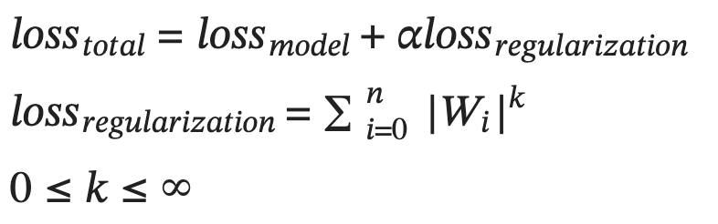 Figure-1: Total loss as a sum of the model loss and regularization loss. k is a floating point value and indicates the regularization norm. Alpha is the weighting factor for the regularization loss.
Typical values of k used in practice are 1 and 2. These are called the L1 and L2 regularization schemes.
But why do we use just these two values for the most part, when in fact there are infinitely many values of k one could use? Let's answer this question with an interpretation of the L1 and L2 regularization schemes.
Interpretation of different weight regularization types
The two most common types of regularization used for machine learning models are L1 and L2 regularization. We will start with these two, and continue to discuss some unusual regularization types such as L0.5 and L3 regularization. We will take a look at the gradients of the regularization losses and plot them to intuitively understand how they affect the model weights.
L1 regularization
L1 regularization adds the average of the absolute value of the weights together as the regularization loss.
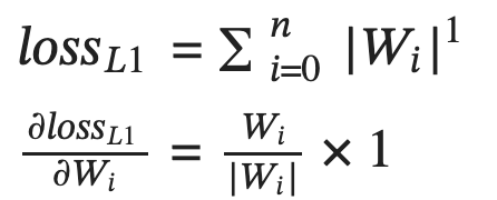 Figure-2: L1 regularization loss and its partial derivative with respect to each weight Wi.
It has the effect of adjusting the weights by a constant (in this case alpha times the learning rate) in the direction that minimizes the loss. Figure 3 shows a graphical representation of the function and its derivative.
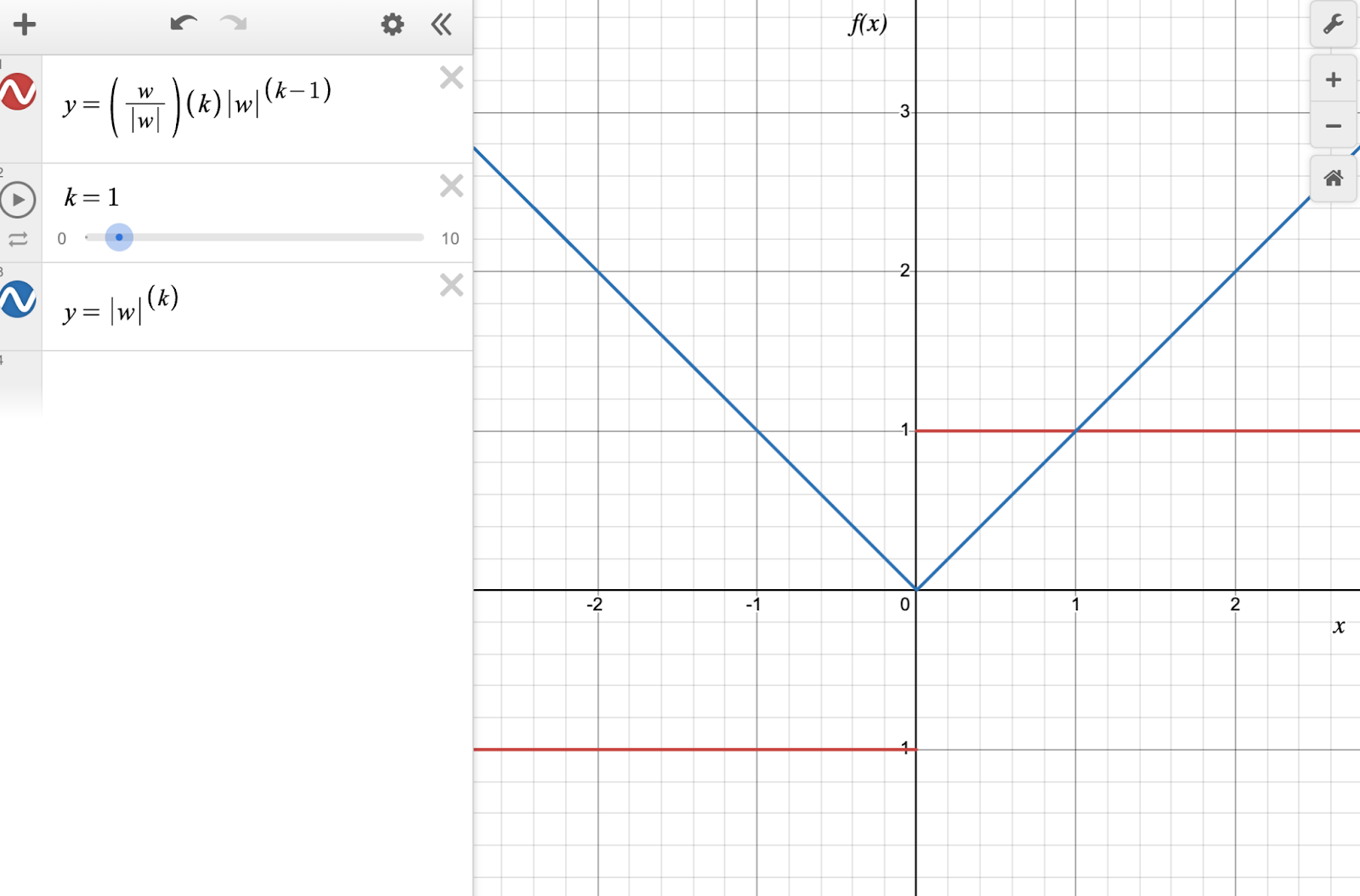 Figure-3: The blue line is |w| and the red line is the derivative of |w|.
You can see that the derivative of the L1 norm is a constant (depending on the sign of w), which means that the gradient of this function only depends on the sign of w and not its magnitude. The gradient of the L1 norm is not defined at w=0.
It means that the weights are moved towards zero by a constant value at each step during backpropagation. Throughout training, it has the effect of driving the weights to converge at zero. That is why the L1 regularization makes a model sparse (i.e. some of the weights become 0). It might cause a problem in some cases if it ends up making a model too sparse. The L2 regularization does not have this side-effect. Let's discuss it in the next section.
L2 regularization
L2 regularization adds the average of the square of the absolute value of the weights together as the regularization loss.
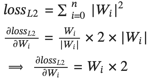 Figure-4: L2 regularization loss and its partial derivative with respect to each weight Wi.
It has the effect of adjusting each weight by a multiple of the weight itself in the direction that minimizes the loss. Figure 5 shows a graphical representation of the function and its derivative.
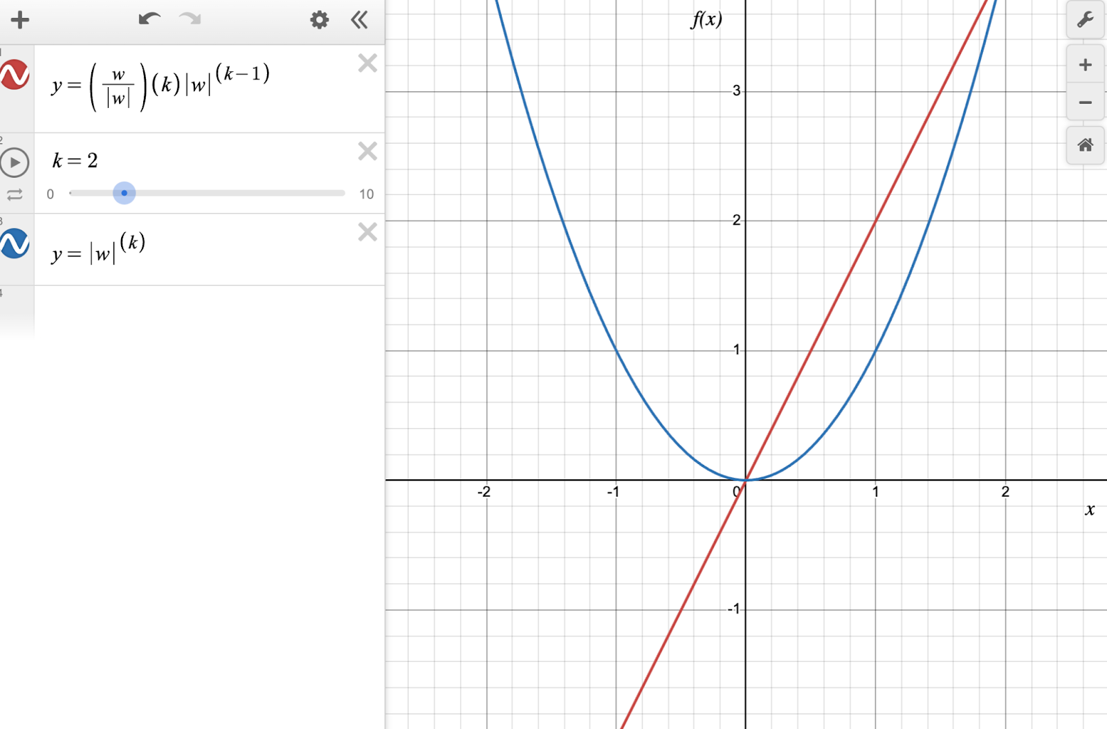 Figure-5: The blue line is pow(|w|, 2) and the red line is the derivative of pow(|w|, 2).
You can see that the derivative of the L2 norm is just the sign-adjusted square root of the norm itself. The gradient of the L2 norm depends on both the sign and magnitude of the weight.
This means that at every gradient update step, the weights will be adjusted toward zero by an amount that is proportional to the weight's value. Over time, this has the effect of drawing the weights toward zero, but never exactly zero, since subtracting a constant factor of a value from the value itself never makes the result exactly zero unless it is zero to begin with. The L2 norm is commonly used for weight decay during machine learning model training.
Let's consider L0.5 regularization next.
L0.5 regularization
L0.5 regularization adds the average of the square root of the absolute value of the weights together as the regularization loss.
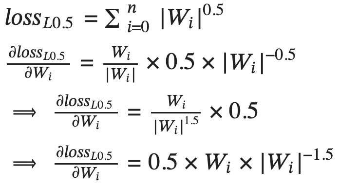 Figure-6: L0.5 regularization loss and its partial derivative with respect to each weight Wi.
This has the effect of adjusting each weight by a multiple (in this case alpha times the learning rate) of the inverse square root of the weight itself in the direction that minimizes the loss. Figure 7 shows a graph of the function and its derivative.
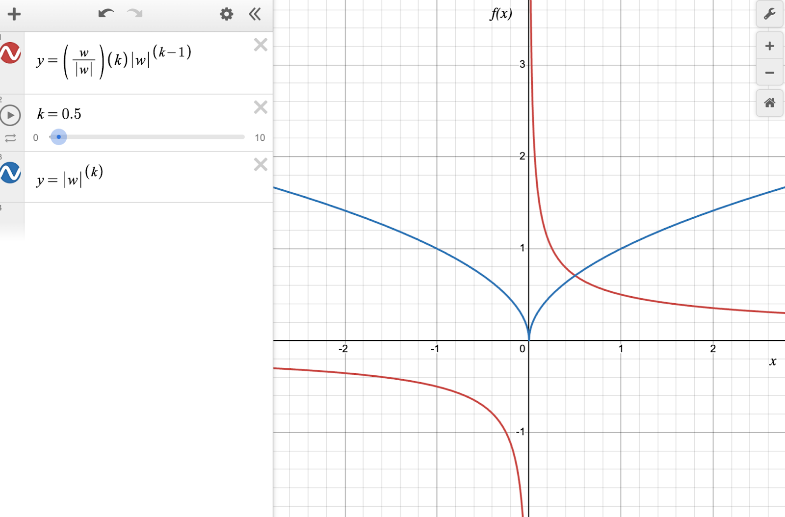 Figure-7: The blue line is pow(|w|, 0.5) and the red line is the derivative of pow(|w|, 0.5).
You can see that the derivative of the L0.5 norm is a discontinuous function, which peaks at the positive values of w close to 0 and it reaches negative infinity for the negative values of w close to 0. Further, we can draw the following conclusions from the graph:
- As |w| tends to 0, the magnitude of the gradient tends to infinity. During backpropagation, these values of w will quickly swing to past 0 because large gradients will cause a large change in the value of w. In other words, negative w will become positive and vice-versa. This cycle of flip flops will continue to repeat itself.
- As |w| increases, the magnitude of the gradient decreases. These values of w are stable because of small gradients. However, with each backpropagation step, the value of w will be drawn closer to 0.
This is hardly what one would want from a weight regularization routine, so it's safe to say that L0.5 isn't a great weight regularizer. Let's consider L3 regularization next.
L3 regularization
L3 regularization adds the average of the cube of the absolute value of the weights together as the regularization loss.
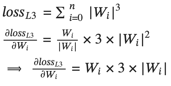 Figure-8: L3 regularization loss and its partial derivative with respect to each weight Wi.
This has the effect of adjusting each weight by a multiple (in this case alpha times the learning rate) of the square of the weight itself in the direction that minimizes the loss.
Graphically, this is what the function and its derivative look like.
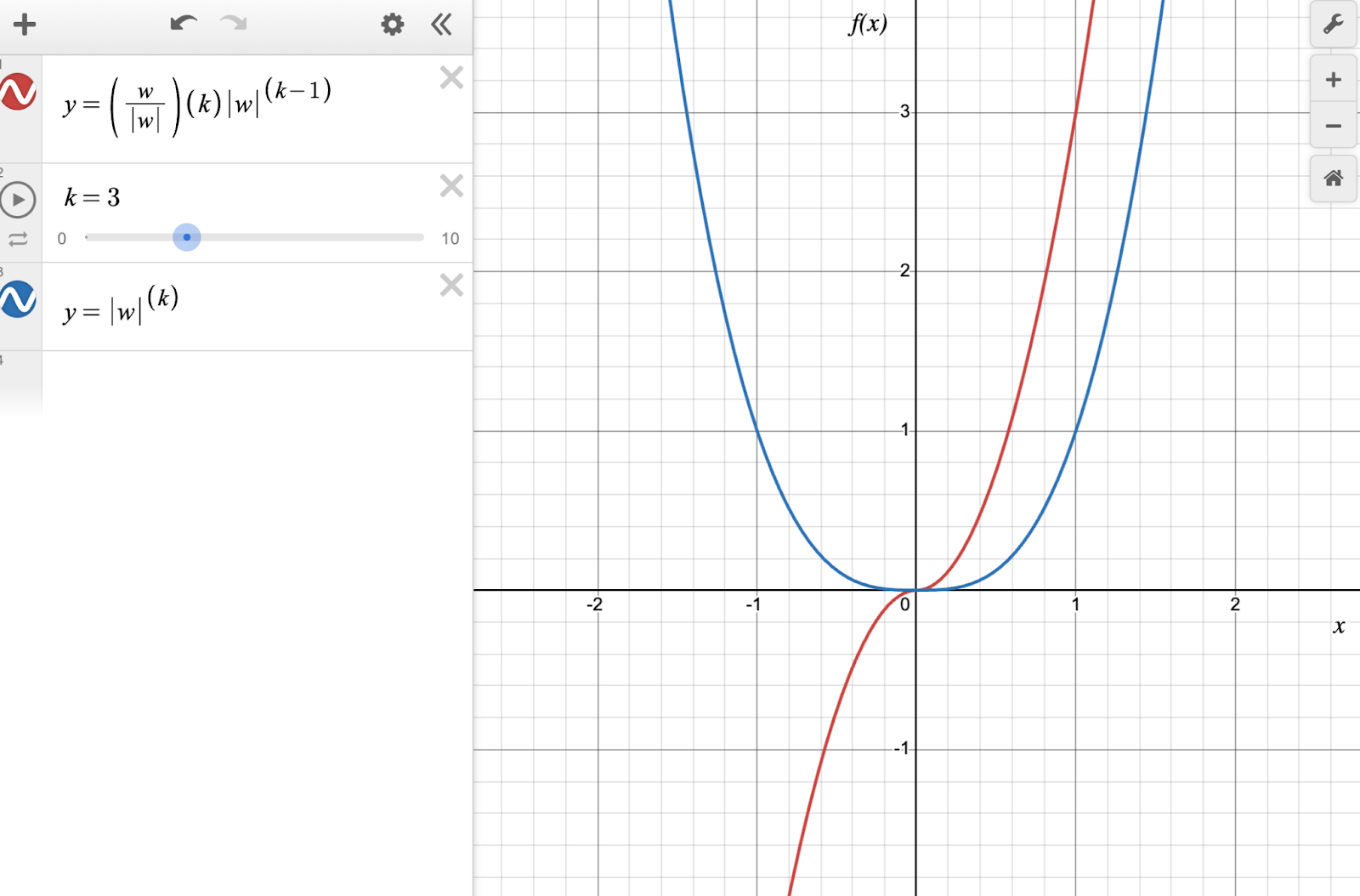 Figure-9: The blue line is pow(|w|, 3) and the red line is the derivative of pow(|w|, 3).
To really understand what's going on here, we need to zoom in to the chart around the w=0 point.
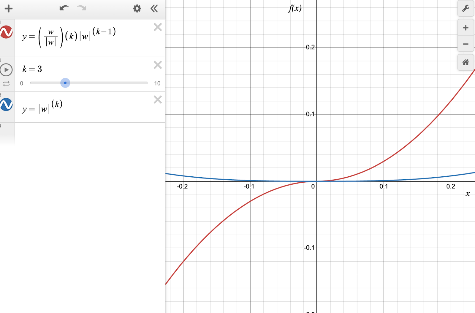 Figure-10: The blue line is pow(|w|, 3) and the red line is the derivative of pow(|w|, 3), zoomed in at small values of w around 0.0.
You can see that the derivative of the L3 norm is a continuous and differentiable function (despite the presence of |w| in the derivative), which has a large magnitude at large values of w and a small magnitude for small values of w.
Interestingly, the gradient is very close to zero for very small values of w around the 0.0 mark.
The interpretation of the gradient for L3 is interesting.
- For large values of w, the magnitude of the gradient is large. During backpropagation, these values will be pushed towards 0.
- Once the weight w reaches an inflection point (close to 0.0), the gradient almost vanishes, and the weights will stop getting updated.
The effect is that it will drive the weights with large magnitudes close to 0, but not exactly 0.
Let's consider higher norms to see how this plays out in the limiting case.
Beyond L3 regularization
To understand what happens for Linfinity, we need to see what happens in the case of the L10 regularization case.
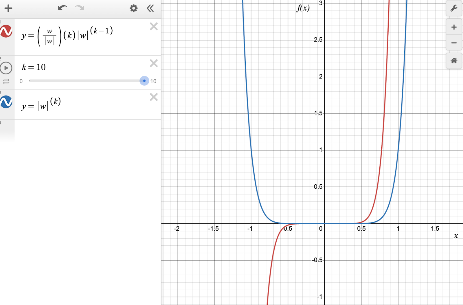 Figure-11: The blue line is pow(|w|, 10) and the red line is the derivative of pow(|w|, 10), zoomed in at small values of w around 0.0.
One can see that the gradients for values of |w| < 0.5 are extremely small, which means that regularization won't be effective for those values of w.
Exercise
Based on everything we saw above, L1 and L2 regularization are fairly practical based on what you want to achieve. As an exercise, try to reason about the behavior of the L1.5 regularization, whose chart is shown below.
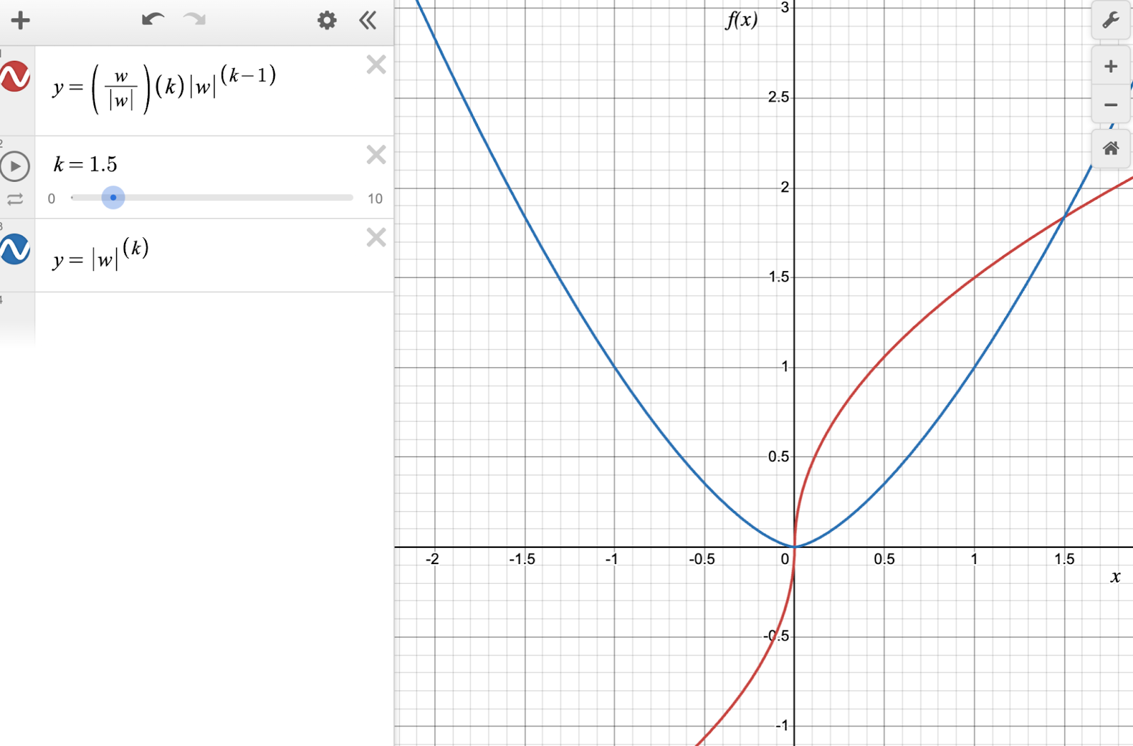 Figure-12: The blue line is pow(|w|, 1.5) and the red line is the derivative of pow(|w|, 1.5).
Conclusion
We took a visual and intuitive look at the L1 and L2 (and in general Lk) regularization terms to understand why L1 regularization results in sparse model weights and L2 regularization results in model weights close to 0. Framing the solution as inspecting the resulting gradients is extremely valuable during this exercise.
We explored L0.5, L3, and L10 regularization terms and graphically, and you (the reader) reasoned about regularization terms between L1 and L2 regularization, and developed an intuitive understanding of what implications it would have on a model's weights.
We hope that this article has added to your toolbox of tricks you can use when considering regularization strategies during model training to fine-tuning.
All the charts in this article were created using the online desmos graphing calculator. Here is a link to the functions used in case you wish to play with them.
All the images were created by the author(s) unless otherwise mentioned.
References
We found the following articles useful while researching the topic, and we hope that you find them useful too!
- Stackexchange discussion
- TDS: Demystifying L1 & L2 Regularization (part 3)
- Visual explanation of L1 and L2 regularization
- Deep Learning by Ian Goodfellow
- An introduction to statistical learning by Gareth James
Register Now to Continue Reading
Unlock Towards Data Science with a Free Account
All articles on Towards Data Science are available to registered users. Create a free account today to access this article and thousands more.
Register for freeSign in to your account
 Written By
See all from Dhruv Matani
Deep Learningl1-and-l2-regularizationMachine LearningRegularizationStatistics
Share This Article
Towards Data Science is a community publication. Submit your insights to reach our global audience and earn through the TDS Author Payment Program.
Write for TDS
Related Articles
Artificial Intelligence
From individual skills to business development, data professionals have many opportunities in the next few years.
Renato Boemer
December 30, 20206 min read
Artificial Intelligence
The need for proper validations and good datasets, objective and balanced, and that predictions be useful in realistic scenarios.
Luciano Abriata
March 14, 202312 min read
Artificial Intelligence
These tips are also applicable to Software Engineers. Make a few changes in your CV...
Roman Orac
April 28, 20214 min read
Machine Learning
Understanding the purpose of requirements.txt, setup.py and setup.cfg in Python when developing and distributing packages
Giorgos Myrianthous
March 1, 20227 min read
Machine Learning
How does regularization work and how can it be used to prevent overfitting?
Ritwick Roy
February 15, 202216 min read
Machine Learning
An End-To-End Tutorial for Beginners
Mike Shakhomirov
October 6, 20239 min read
Artificial Intelligence
How to find the underlying structure of data
Soner Yıldırım
April 23, 20209 min read
Artificial Intelligence
Hands-on ReAct agent implementation with AdalFlow library
Li Yin
July 14, 202415 min read
Machine Learning
Avoid trial and error-based dataset size estimation for your next ML project.
Shashank Deshpande
June 4, 202110 min read
Your home for data science and AI. The world's leading publication for data science, data analytics, data engineering, machine learning, and artificial intelligence professionals.
Subscribe to Our NewsletterWrite For TDS•About•Advertise•Privacy Policy•Terms of Use
© Insight Media Group, LLC 2026•The New Stack•roadmap.sh•Creator Network
Recommended Articles
Close