保留正文与补采附件。源页面当前未重新核验;具体限制见交付清单。
 We value your privacy
We use cookies to enhance your browsing experience, serve personalised ads or content, and analyse our traffic. By clicking "Accept All", you consent to our use of cookies.
Customise Reject All Accept All
Customise Consent Preferences
 We use cookies to help you navigate efficiently and perform certain functions. You will find detailed information about all cookies under each consent category below.
The cookies that are categorised as "Necessary" are stored on your browser as they are essential for enabling the basic functionalities of the site. ... Show more
NecessaryAlways Active
Necessary cookies are required to enable the basic features of this site, such as providing secure log-in or adjusting your consent preferences. These cookies do not store any personally identifiable data.
-
Cookie
BCTempID
-
Duration
10 minutes
-
Description
No description available.
-
Cookie
__cf_bm
-
Duration
1 hour
-
Description
This cookie, set by Cloudflare, is used to support Cloudflare Bot Management.
-
Cookie
AWSALBCORS
-
Duration
7 days
-
Description
Amazon Web Services set this cookie for load balancing.
-
Cookie
_cfuvid
-
Duration
session
-
Description
Cloudflare sets this cookie to track users across sessions to optimize user experience by maintaining session consistency and providing personalized services
-
Cookie
li_gc
-
Duration
6 months
-
Description
Linkedin set this cookie for storing visitor's consent regarding using cookies for non-essential purposes.
-
Cookie
__hssrc
-
Duration
session
-
Description
This cookie is set by Hubspot whenever it changes the session cookie. The __hssrc cookie set to 1 indicates that the user has restarted the browser, and if the cookie does not exist, it is assumed to be a new session.
-
Cookie
__hssc
-
Duration
1 hour
-
Description
HubSpot sets this cookie to keep track of sessions and to determine if HubSpot should increment the session number and timestamps in the __hstc cookie.
-
Cookie
wpEmojiSettingsSupports
-
Duration
session
-
Description
WordPress sets this cookie when a user interacts with emojis on a WordPress site. It helps determine if the user's browser can display emojis properly.
-
Cookie
BCSessionID
-
Duration
1 year 1 month 4 days
-
Description
Blueconic sets this cookie as a unique identifier for the BlueConic profile.
-
Cookie
_octo
-
Duration
1 year
-
Description
No description available.
-
Cookie
logged_in
-
Duration
1 year
-
Description
No description available.
-
Cookie
__Secure-YEC
-
Duration
past
-
Description
YouTube sets this cookie to stores the user's video player preferences using embedded YouTube video
-
Cookie
__eoi
-
Duration
6 months
-
Description
Description is currently not available.
-
Cookie
AWSALBTGCORS
-
Duration
7 days
-
Description
No description available.
-
Cookie
login-status-p
-
Duration
past
-
Description
Description is currently not available.
-
Cookie
AWSALBTG
-
Duration
7 days
-
Description
No description available.
-
Cookie
csrf_token
-
Duration
session
-
Description
No description available.
-
Cookie
token_v2
-
Duration
1 day
-
Description
Description is currently not available.
-
Cookie
D
-
Duration
1 year
-
Description
Description is currently not available.
-
Cookie
PHPSESSID
-
Duration
session
-
Description
This cookie is native to PHP applications. The cookie stores and identifies a user's unique session ID to manage user sessions on the website. The cookie is a session cookie and will be deleted when all the browser windows are closed.
-
Cookie
VISITOR_PRIVACY_METADATA
-
Duration
6 months
-
Description
YouTube sets this cookie to store the user's cookie consent state for the current domain.
-
Cookie
cookietest
-
Duration
session
-
Description
The cookietest cookie is typically used to determine whether the user's browser accepts cookies, essential for website functionality and user experience.
-
Cookie
__Host-airtable-session
-
Duration
1 year
-
Description
This cookie is used to enable us to integrate the services of Airtable.
-
Cookie
__Host-airtable-session.sig
-
Duration
1 year
-
Description
This cookie is used to enable us to integrate the services of Airtable.
-
Cookie
m
-
Duration
1 year 1 month 4 days
-
Description
Stripe sets this cookie for fraud prevention purposes. It identifies the device used to access the website, allowing the website to be formatted accordingly.
-
Cookie
BIGipServer*
-
Duration
session
-
Description
Marketo sets this cookie to collect information about the user's online activity and build a profile about their interests to provide advertisements relevant to the user.
-
Cookie
__cfruid
-
Duration
session
-
Description
Cloudflare sets this cookie to identify trusted web traffic.
-
Cookie
_GRECAPTCHA
-
Duration
6 months
-
Description
Google Recaptcha service sets this cookie to identify bots to protect the website against malicious spam attacks.
-
Cookie
__Secure-YNID
-
Duration
6 months
-
Description
Google cookie used to protect user security and prevent fraud, especially during the login process.
-
Cookie
cookieyes-consent
-
Duration
1 year
-
Description
CookieYes sets this cookie to remember users' consent preferences so that their preferences are respected on subsequent visits to this site. It does not collect or store any personal information about the site visitors.
Functional
Functional cookies help perform certain functionalities like sharing the content of the website on social media platforms, collecting feedback, and other third-party features.
-
Cookie
lidc
-
Duration
1 day
-
Description
LinkedIn sets the lidc cookie to facilitate data center selection.
-
Cookie
brw
-
Duration
1 year
-
Description
No description available.
-
Cookie
brwConsent
-
Duration
5 minutes
-
Description
Description is currently not available.
-
Cookie
WMF-Uniq
-
Duration
1 year
-
Description
Description is currently not available.
-
Cookie
loom_anon_comment
-
Duration
1 year
-
Description
No description available.
-
Cookie
loom_referral_video
-
Duration
session
-
Description
Description is currently not available.
-
Cookie
VISITOR_INFO1_LIVE
-
Duration
6 months
-
Description
A cookie set by YouTube to measure bandwidth that determines whether the user gets the new or old player interface.
-
Cookie
yt-remote-connected-devices
-
Duration
Never Expires
-
Description
YouTube sets this cookie to store the user's video preferences using embedded YouTube videos.
-
Cookie
ytidb::LAST_RESULT_ENTRY_KEY
-
Duration
Never Expires
-
Description
The cookie ytidb::LAST_RESULT_ENTRY_KEY is used by YouTube to store the last search result entry that was clicked by the user. This information is used to improve the user experience by providing more relevant search results in the future.
-
Cookie
yt-remote-device-id
-
Duration
Never Expires
-
Description
YouTube sets this cookie to store the user's video preferences using embedded YouTube videos.
-
Cookie
yt-remote-session-name
-
Duration
session
-
Description
The yt-remote-session-name cookie is used by YouTube to store the user's video player preferences using embedded YouTube video.
-
Cookie
yt-remote-fast-check-period
-
Duration
session
-
Description
The yt-remote-fast-check-period cookie is used by YouTube to store the user's video player preferences for embedded YouTube videos.
-
Cookie
yt-remote-session-app
-
Duration
session
-
Description
The yt-remote-session-app cookie is used by YouTube to store user preferences and information about the interface of the embedded YouTube video player.
-
Cookie
yt-remote-cast-available
-
Duration
session
-
Description
The yt-remote-cast-available cookie is used to store the user's preferences regarding whether casting is available on their YouTube video player.
-
Cookie
yt-remote-cast-installed
-
Duration
session
-
Description
The yt-remote-cast-installed cookie is used to store the user's video player preferences using embedded YouTube video.
-
Cookie
cp_session
-
Duration
3 months
-
Description
Codepen sets this cookie for Help systems found in the website.
-
Cookie
loid
-
Duration
1 year 1 month 4 days
-
Description
This cookie is set by the Reddit. The cookie enables the sharing of content from the website onto the social media platform.
Analytics
Analytical cookies are used to understand how visitors interact with the website. These cookies help provide information on metrics such as the number of visitors, bounce rate, traffic source, etc.
-
Cookie
__hstc
-
Duration
6 months
-
Description
Hubspot set this main cookie for tracking visitors. It contains the domain, initial timestamp (first visit), last timestamp (last visit), current timestamp (this visit), and session number (increments for each subsequent session).
-
Cookie
hubspotutk
-
Duration
6 months
-
Description
HubSpot sets this cookie to keep track of the visitors to the website. This cookie is passed to HubSpot on form submission and used when deduplicating contacts.
-
Cookie
_ga
-
Duration
1 year 1 month 4 days
-
Description
Google Analytics sets this cookie to calculate visitor, session and campaign data and track site usage for the site's analytics report. The cookie stores information anonymously and assigns a randomly generated number to recognise unique visitors.
-
Cookie
ga*
-
Duration
1 year 1 month 4 days
-
Description
Google Analytics sets this cookie to store and count page views.
-
Cookie
__Host-psifi.analyticsTrace
-
Duration
6 hours
-
Description
Description is currently not available.
-
Cookie
__Host-psifi.analyticsTraceV2
-
Duration
6 hours
-
Description
Description is currently not available.
-
Cookie
_gh_sess
-
Duration
session
-
Description
GitHub sets this cookie for temporary application and framework state between pages like what step the user is on in a multiple step form.
-
Cookie
YSC
-
Duration
session
-
Description
YSC cookie is set by Youtube and is used to track the views of embedded videos on Youtube pages.
-
Cookie
ajs_anonymous_id
-
Duration
1 year
-
Description
This cookie is set by Segment to count the number of people who visit a certain site by tracking if they have visited before.
-
Cookie
vuid
-
Duration
1 year 1 month 4 days
-
Description
Vimeo installs this cookie to collect tracking information by setting a unique ID to embed videos on the website.
Performance
Performance cookies are used to understand and analyse the key performance indexes of the website which helps in delivering a better user experience for the visitors.
-
Cookie
AWSALB
-
Duration
7 days
-
Description
AWSALB is an application load balancer cookie set by Amazon Web Services to map the session to the target.
-
Cookie
acq
-
Duration
past
-
Description
Description is currently not available.
-
Cookie
acq.sig
-
Duration
past
-
Description
Description is currently not available.
-
Cookie
ptc
-
Duration
2 years
-
Description
No description available.
Advertisement
Advertisement cookies are used to provide visitors with customised advertisements based on the pages you visited previously and to analyse the effectiveness of the ad campaigns.
-
Cookie
muc_ads
-
Duration
1 year 1 month 4 days
-
Description
Twitter sets this cookie to collect user behaviour and interaction data to optimize the website.
-
Cookie
guest_id_marketing
-
Duration
1 year 1 month 4 days
-
Description
Twitter sets this cookie to identify and track the website visitor.
-
Cookie
guest_id_ads
-
Duration
1 year 1 month 4 days
-
Description
Twitter sets this cookie to identify and track the website visitor.
-
Cookie
personalization_id
-
Duration
1 year 1 month 4 days
-
Description
Twitter sets this cookie to integrate and share features for social media and also store information about how the user uses the website, for tracking and targeting.
-
Cookie
guest_id
-
Duration
1 year 1 month 4 days
-
Description
Twitter sets this cookie to identify and track the website visitor. It registers if a user is signed in to the Twitter platform and collects information about ad preferences.
-
Cookie
bcookie
-
Duration
1 year
-
Description
LinkedIn sets this cookie from LinkedIn share buttons and ad tags to recognize browser IDs.
-
Cookie
__Secure-ROLLOUT_TOKEN
-
Duration
6 months
-
Description
YouTube sets this cookie to manage feature rollout and experimentation. It helps Google control which new features or interface changes are shown to users as part of testing and staged rollouts, ensuring consistent experience for a given user during an experiment.
-
Cookie
yt.innertube::nextId
-
Duration
Never Expires
-
Description
YouTube sets this cookie to register a unique ID to store data on what videos from YouTube the user has seen.
-
Cookie
yt.innertube::requests
-
Duration
Never Expires
-
Description
YouTube sets this cookie to register a unique ID to store data on what videos from YouTube the user has seen.
-
Cookie
session_tracker
-
Duration
session
-
Description
This cookie is set by the Reddit. This cookie is used to identify trusted web traffic. It also helps in adverstising on the website.
-
Cookie
edgebucket
-
Duration
session
-
Description
Reddit sets this cookie to save the information about a log-on Reddit user, for the purpose of advertisement recommendations and updating the content.
-
Cookie
did
-
Duration
1 year
-
Description
Arbor sets this cookie to show targeted ads to site visitors.This cookie expires after 2 months or 1 year.
Uncategorised
Other uncategorised cookies are those that are being analysed and have not been classified into a category as yet.
No cookies to display.
Reject All Save My Preferences Accept All
Toggle SearchToggle Mobile Navigation
Publish AI, ML & data-science insights to a global community of data professionals.
Sign inSubmit an Article
LatestEditor's PicksNewsletterShipAI
Write For TDS
LinkedInXToggle Search
Machine Learning
An Introduction to Supervised Learning
The one with an example of the Naive Bayes classification algorithm
James Andrew Godwin
February 26, 202223 min read
 caption | Photo by Anni Roenkae
This continues a series of articles that build on each other. Please read my last article on Time Series Analysis and Logistic Regression.
Alright, let us start with supervised learning. I covered some of this in my earlier articles but let me go over some specifics for this article.
- Supervised learning: learns from existing data which are categorized and labeled with predefined classes. Test data are labeled into these classes as well
Well, this is true of all types of learning. But, specifically, it has labeled predefined classes. That is the most important thing - supervised learning has something that is called an expert label. That's a fancy word for meaning that it is labeled for an outcome; or for any given case, there is a known, desired outcome.
Unsupervised learning (clustering) does not assume that it knows the answer. So clustering, for instance, will take a look at the data and partition the data, according to how the data are.
Learn this step by step with the interactive Machine Learning roadmap.
Supervised learning will partition the data according to the label. This is a big difference. An example of unsupervised learning is clustering. An example of supervised learning is regression, as I have written about before.
For instance, in a regression model, we have X and Y, and we draw a best fit line through that. In this example, X are our inputs, and Y is the output. We can say this is supervised learning because Y is the expert label; the model is learning how to take X and come up with Y given these expert labels.
Examples:
- Fraud transaction: we know which transactions in the training data were fraud (1), and which were not (0)
- Readmission: we know which patients were readmitted to a hospital within a certain time window after discharge
- Recommendation: we know which items were presented to customers, and which items were clicked, added to the cart, or purchased
- A classic example is a spam filter
Machine learning tasks have a variety of purposes. Here are a few examples of classic machine learning tasks: identifying fraud, identifying readmission of patients, identifying recommendations like your typical Netflix machine learning case that is when you go on to Netflix, you get recommendations of movies that you will like; those movies are based on previous movies that you looked at and considering what other people liked when they had watched similar movies to the movies you watched, and what movies they watched, in addition to that. This is called a recommendation engine.
As an aside, this recommendation engine is sort of a gray area, that might not always be described as supervised learning, but I digress.
A classic example of supervised learning is a spam filter. What does a spam filter do? It classifies between spam and no spam on your email. The way the model learned this is by someone, an "expert" - a human, who came by and marked various emails as spam or not spam. Then the emails and those labels were given to an algorithm that was expected to figure out how to get from the email to that label on its own. This whole process is called supervised learning.
Typical machine learning tasks:
- Classification: can we label the input?
- Regression : can we make a prediction?
- Recommendations : can we predict something based on user preference?
Supervised learning has two important steps: first, you train a model, and then you test the model. It is very important to use unseen test data for testing your model. In previous articles, I wrote about supervised learning, like with a regression, I did not use test data, and used training data to test the model. This is is bad, not a good thing to do. People do it on occasion, there are different reasons for doing it. There are very few legitimate reasons, but there are some. If you use training data to determine the accuracy of your model, then you are at best fooling yourself; and at worst, you are lying.
So to test the model, you need to use so-called "unseen test data." Now, how do we create unseen test data? Well, that is pretty simple. You just take your modeling data and split it into training data and test data: the test data is used for the testing of the model after the model has been trained on the training segment.
What do we mean by learning? You use the data together with the algorithm to come up with a performance measure or to minimize a cost function - that is the other way of saying it. When you do that, then you will come up with a model with new operational data and you will be able to get an answer.
Fundamental assumption of learning
A fundamental assumption of learning is that the distribution of training examples is identical to the distribution of test examples, including future unseen examples. More importantly, the distribution of training examples is similar enough to future examples. Given that they are future examples, they are unseen.
If you want to have an accuracy measure, then that distribution should also be similar to the test examples. This assumption is not a requirement. What is a requirement is that your test examples, for you to trust your accuracy, have to come from the same distribution as your future examples.
Where your training examples came from is not important if you create a usable model. If your training examples come from a different distribution, more power to you. To be a valid measure, the test examples have to be similar enough to the examples that will be used in practice when it comes to operational data - when it comes to operationalizing. Now strong violations to the above assumption will result in poor classification accuracy.
Machine learning framework
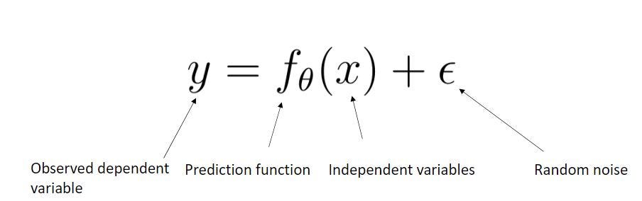 Image by author
Training: given a training set of labeled examples {(x_1, y_1, ... (x_n, y_n)}, estimate the prediction function (f) and parameters (Theta) which minimizes the prediction error on the training set
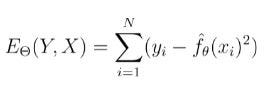 Training function | Image by author
Testing: apply (f) to a never before seen test example (x) and output the predicted value (y = f(x))
With the overall machine learning framework, you give an X and you get back a Y. And there is going to be somewhat of an error because there is some random noise associated with everything. That means that the actual Y that you get is not going to be exactly the above function.
Classification Workflow
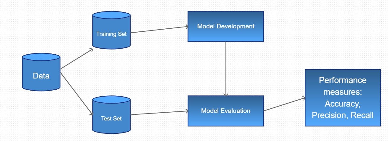 Classification workflow diagram | Image by author
The most important thing is the data have to be split into a training set and test set. The model is developed in the training set, the model is evaluated on the test set. Lastly, you get performance measures, also called accuracy measures. Here there are three performance measures: of which the performance measure called accuracy is probably the worst performance measure. Precision and recall are pretty good. There is a better one that is a hybrid of precision and recall, the F1 score.
The reason I like it more is that it is sort of a hybrid between the recall and the precision. And you will want to have both good recall and precision. If you have very good recall and very lousy precision or vice versa, your model is not worth much. There is an even better accuracy measure for binary classifications - the ROC AUC.
So the AUC, area under the curve, of a ROC curve, is for classifications. The reason why it is better than the previous performance measures is that it is valid for all thresholds; whereas accuracy or precision presumes a threshold - typically it presumes a threshold of 0.5. Likewise, the F1 score also presumes a threshold of 0.5. You could choose a different threshold, but most people would not assume that you would have chosen a different threshold.
The reason why you choose a different threshold is that you may have a different purpose in mind, where you have false positives might be worse for you than false negatives, or vice versa. By being able to tune your threshold, you can trade those off.
Many classifiers to choose from
- Linear Regression
- Logistic Regression
- Support Vector Machine (SVM)
- Neural networks (ANN, CNN, RNN, DNN)
- Naive Bayes
- Bayesian network
- Randomized Forests (Random forests)
- Boosted Decision Trees (Gradient boosted trees)
- K-nearest neighbor (KNN)
Here are so-called classifiers, algorithms used in supervised learning. KNN is generally considered your simplest concept and is often taught in classes like these because the algorithm is relatively simple: you can write out the algorithm from scratch.
Boosted decision trees and randomized forests used to be your generally favored machine learning classification algorithms. Today the "newest" types of algorithms are the neural nets. And when I say the newest, my statement is about five to 10 years old, depending on how you look at it. But up to about five years ago, Kaggle competitions were won by boosted decision trees and randomized forests. Now Kaggle competitions are being won by deep neural nets. So not neural nets, as such, but a more sophisticated version of neural nets called deep neural nets (DNN).
Logistic regression is everyone's favorite - whenever you do a classification, you first do a logistic regression, always! Naive Bayes is a favorite too in that same sense. But logistic regression maybe even a little bit more so. So you always do logistic regression; not because you want to show off the results of the logistic regression. It is just that it is so robust and you know if you cannot get the logistic regression to work, you will not be able to get anything else to work either. So logistic regression is the first thing you try to get to work. When that works, then you start becoming more daring and venture into some of these other algorithms listed above.
Generalization
Underfitting : model is too "simple" to represent all the relevant class characteristics - high training error and high validation error.
Overfitting : model is too "complex" and fits irrelevant characteristics (noise) in the data - low training error and high validation error (big gap between training and validation performance)
Generalization means how well it works. As a good heuristic whenever you say generalization, you think of regularization. Why do this? Because the way you generalize a model is by regularizing the model. If you have a well-regularized model, it is presumably generalized. What does generalization mean? It means it will work under more than just minimal circumstances. Thus no overfitting has occurred. An underfit model is generally too simple and more work needs to be done to extract information from it. But an overfit model is not generalized well enough and requires regularization.
Common pitfalls in machine learning
- Overfitting
- Underfitting
- Data leakage : the creation of unexpected additional information in the training data, creating unrealistically good predictions. Leaking test data into training data. The inclusion of data not present in the model's operational environment
Rarely is underfitting a pitfall, maybe the usage of algorithms which are too primitive and that results in sort of a way of underfitting because people might have stopped with logistic regression and they should have used a gradient boosted tree if you want to consider that a kind of underfitting. Overfitting is one of your big issues, as mentioned earlier.
Now the next big issue is data leakage or proxy columns or proxies of any sort. These issues happen a lot. This concept is hard to understand, it is hard to explain, hard to teach why such things happen often unless you have done this yourself.
For example, where you have been looking at your data for a month, working with it, and only once your test results come back, and you see your test results for your machine learning algorithm like .97 on your accuracy. Only then do you realize, "Oh, I must have data leakage." Simply put - it is vanishingly rare that you get a model that good. Then you have to dissect your model, you have to find out why your model is too good to be true. And the reason your model is too good to be true is usually because of data leakage.
A real-life example: a prostate cancer model included a variable stating whether or not patients had prostate cancer surgery. A model cannot see the future, and the data for whether or not the patient had surgery should have been removed from the model for training.
Confusion Matrix
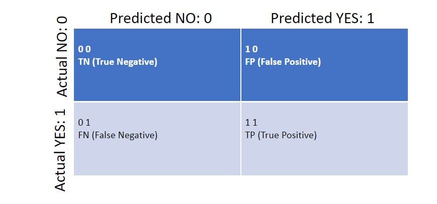 Encoding for the confusion matrix
Here is an example of a confusion matrix. One important note about these confusion matrices is that they typically have the true negative in the upper left and the true positive in the lower right. The reason why this is the case, nowadays, is because zero is less than one. Since true negatives are usually modeled as zeros, it makes numeric sense to list them first. When you have your actual versus your predicted classes reduced to the easiest format for a computer to understand them, then you have reduced them to zero and one. Since zero is smaller than one zero goes first and one goes second. Since zeros are smaller than one, zeros go first also in the vertical dimension and then ones well. Zeros are typically associated with the absence of something and they are typically associated with a negative.
Here a negative is not a bad thing - if I am COVID-19 negative, this means I do not have COVID, or at least my test came back negative for COVID. If I do not have COVID then this is what I call a true negative or 0 0. Likewise, the encoding of 1 1 would mean I do have COVID and I tested positive for it.
This is why true negatives and true positives are aligned this way: true negatives are in the upper left, true positives are in the lower right. This was not always the case - it used to be the other way around! But this is what you see most of the time these days. And that just has to do with the ordering of zero and one!
Precision and recall are important concepts to understand but are beyond the scope of this article. As I mentioned above, I prefer the F1 score, the harmonic mean (as opposed to the arithmetic mean) of precision and recall as my "accuracy" metric over choosing either one. But the best performance measure for classification is the ROC curve.
The Receiver Operating Characteristic (ROC) curve is great for classifications. I believe it is the most important accuracy measure but sometimes it cannot be used. There are reasons for that, but generally, the ROC curve is what you want to use. The reason why you want to use the ROC curve is that it considers all thresholds. To illustrate why this is important, consider this hypothetical interview question: give people numbers for false positive, for true positive, false negative, and true negative - there are there 10 in each of those. So that would give you about the worst accuracy score possible: 0.5
as an aside consider that if your model is .01 accurate, then just switch the labels for your 0 and 1 classes and suddenly your model is .99 accurate
But if you look at the probabilities, the probabilities for the true positives and the true negatives: are all-around zero and one - meaning they are good. The probabilities of the false positives and false negatives are all around 0.5, which means they are really bad. This means the errors are shaky, and the correct results are very good or very secure; thus you will get a higher ROC AUC score for that! You will never see anything like that with any of these other accuracy measures because they do not consider probabilities. They only consider the boolean outcomes : is it a true positive or is it not a true positive?
Naive Bayes
Some properties of Naive Bayes models are
- Do not require a prior
- Computational complexity is linear in the number of parameters/features
- Requires minimal data to produce models that generalize well
- Have a simple and inherent regularization
Some applications:
- Document classification
- SPAM detection
- Image classification
Yes, the Bayes in Naive Bayes does refer to Bayes theorem, which I have previously written about. There is also a very clear link between Bayes theorem and Naive Bayes model. However, the presumption with the Naive Bayes model is that the individual dimensions are independent, or naive. That means the important part about Bayes theorem, where you can relate the probability of A to the probability of B or the intersection is not needed. What we have here in the naive consideration is that we say that these probabilities are independent of each other. Thus the conditional probability basically goes away. This is the "naive" in Naive Bayes - acting as if your data dimensions are independent.
If your data dimensions are not independent, then your Naive Bayes will not work well. A surprising result, or at least surprising if you focus too much on this independence requirement, is that the Naive Bayes model will still work pretty well if your dimensions are not fully independent. Regardless my point is that some of the most difficult parts in considering Bayes theorem become very simple with Naive Bayes; because you presume that the probabilities are independent of each other - thus no conditional probabilities need to be calculated or presumed. The dimensional independence presumption allows you to multiply probabilities with each other, which greatly simplifies the computations needed to train and test the model.
Like how a logistic regression is used as a classifier, you would not be wrong to call it, instead, a logistic classifier. Thus a better name for Naive Bayes might be the Naive Probability Model, to distance itself from the conditional probabilities inherent in Bayes theorem.
Pitfalls of Naive Bayes
- Multiplication of small probabilities leads to floating-point underflow. This problem is corrected by computing with the log probabilities, ln(p)
- If there are no samples/data then p(xj | Ck) = 0, leading to the product of the probabilities to be 0. A Laplace smoother is used to ensure that all p(xj | Ck) > 0
- Collinear features do not exhibit independence. Ideally, such features should be removed from the dataset to prevent problems with the model
- Regularization is generally a minor issue with Naive Bayes models, as uninformative features tend to a uniform distribution, which does not affect the outcome
Types of Naive Bayes Models
Now that we have looked into the basics of a Naive Bayes model, let us look at some specific formulations. It is important to keep in mind that a specific naive Bayes model is required for each class of problems.
The multinomial naive Bayes classifier is a widely used form of the model. The multinomial classifier finds the most likely class from multiple possibilities. To prevent numerical underflow we write this classifier taking the logarithms of both sides of the equation as follows:
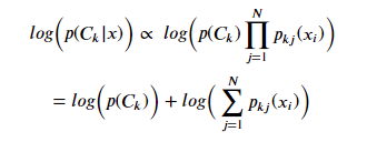 Image by author
The most likely class 𝑦̂ is then:
 Image by author
The multinomial classifier can be simplified for the Bernoulli or binary case as:
 Image by author
Document Classification Example
- The Naive Bayes topic model computes the probability that document D has topic C based on the occurrence of the words {w1, w2,..., wn}, using the following relationship:
 Credit: Wikipedia
In this document classification example, you have a variety of documents, a so-called corpus of documents. That means you have a collection of documents and these documents are labeled in some way. First, a document is given an "expert" label (spam or not spam). After applying labels what you do is you create a column out of every word, which means every word becomes a boolean column, like with one-hot encoding.
You repeat this process for every word in that document. There are ways of reducing the number of columns but my point is that Naive Bayes is very useful for document classification. Now, what are some examples of this? For instance, is this document plagiarized or not? Is this document fake news or not? Is this spam or not? The reason why Naive Bayes is a favored method is that the model does not mind the huge number of dimensions. There can be some performance degradation or fidelity degradation resulting in the classifier not having as good accuracy with huge numbers of data dimensions. But, there are ways of removing superfluous inputs. Computationally speaking, this is very quick hence why it is a favorite choice for document classification.
Python Code Example
Now that the theory has been laid let me walk you through a practical example. What follows is a simple example of a Naive Bayes model. Consider the HouseVotes84which contains political party and votes on 16 important bills for 435 members of the US House of Representatives in 1984.
I will use this data set to build and test a classifier to predict the political party of the congresspeople. Let us begin with the imports:
text
import pandas
import numpy
import seaborn
from matplotlib import pyplot
text
%matplotlib inline
text
votes = pandas.read_csv('https://library.startlearninglabs.uw.edu/DATASCI410/Datasets/house-votes-84.csv', header=None,
names=['class', 'V1', 'V2', 'V3', 'V4', 'V5', 'V6', 'V7', 'V8', 'V9','V10', 'V11', 'V12', 'V13', 'V14', 'V15', 'V16'])
print(votes.shape)
votes.head()
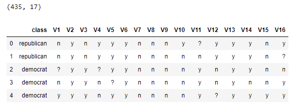 Shape and first 5 rows of dataset | Image by author
Assigning Topics
Each of the vote columns in the above data frame corresponds to the following topics, so let us replace the column names with something easier to remember:
text
vote_names = [
    'handicapped_infants',
    'water_project_cost_sharing',
    'adoption_of_the_budget_resolution',
    'physician_fee_freeze',
    'el_salvador_aid',
    'religious_groups_in_schools',
    'anti_satellite_test_ban',
    'aid_to_nicaraguan_contras',
    'mx_missile',
    'immigration',
    'synfuels_corporation_cutback',
    'education_spending',
    'superfund_right_to_sue',
    'crime',
    'duty_free_exports',
    'export_administration_act_south_africa']
text
votes.columns = ['class'] + vote_names
votes.head()
 Relabled columns | Image by author
Visual exploration - Bar Plots
To further understand this data, let's make some plots of the first 5 votes. The code in the cell below creates bar plots for these votes by Class political parties. Execute this code and examine the results:
text
# Convert dataframe columns to "category" type to take advantage
# categorical utilities like facet-based plotting in seaborn
text
votes['class'] = pandas.Categorical(votes['class'].astype('object')
    , categories=['republican', 'democrat'])
text
values = ['y', 'n', '?']
vote_dtype = pandas.api.types.CategoricalDtype(categories=values)
for c in votes.columns[1:]:
    votes[c] = votes[c].astype('object').astype(
        vote_dtype)
democrats = votes[votes['class'] == 'democrat']
republicans = votes[votes['class'] == 'republican']
for vote_col in votes.columns[1:6]:
    pyplot.subplot(1, 2, 1)
    pyplot.hist([1 if x == 'y' else 0 for x in democrats[vote_col]])
    pyplot.title('Democrats: n' + vote_col)
    pyplot.ylabel('count')
    pyplot.subplot(1, 2, 2)
    pyplot.hist([1 if x == 'y' else 0 for x in republicans[vote_col]])
    pyplot.title('Republicans: n' + vote_col)
    pyplot.show()
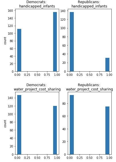 Image by author
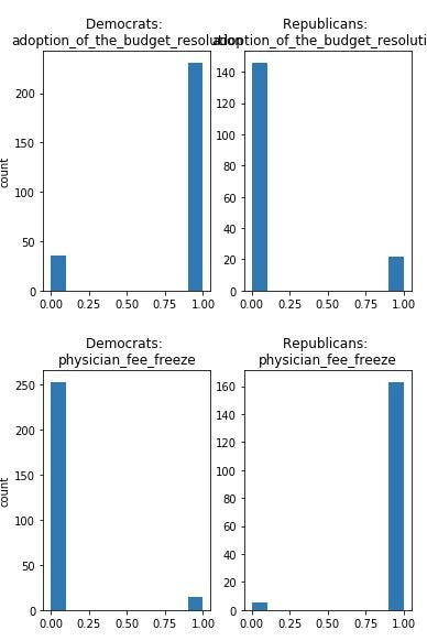 Image by author
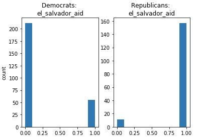 Image by author
When examining these charts, keep in mind that there are more Democrats than Republicans in this data set - thus it is not perfectly balanced. What is important is the probability of a Yes vote or No vote for the members of each party. Some votes are quite skewed by party affiliation, such as 'adoption of the budget resolution'. Whereas, some votes have similar probabilities by party, such as 'water project cost sharing'. These probabilities of votes by political party are used to train the Naive Bayes model.
Train and Test the Model
Now that we understand a bit about the characteristics of the data, it's time to train and test a naive Bayes model. The python sklearn.naive_bayes package provides a library that trains a naive Bayes model and produces a model object that can make predictions on new instances:
text
import sklearn.model_selection as m_s
Votes_Train, Votes_Test = m_s.train_test_split(votes)
votes = Votes_Test
text
label_col = 'class'
text
# Convert our categorical values to numeric feature vectors
feature_vecs = numpy.array([
        votes[c].cat.codes
        for c in votes.columns
        if c != label_col]).T
print(feature_vecs.shape)
text
feature_Train = numpy.array([
        Votes_Train[c].cat.codes
        for c in Votes_Train.columns
        if c != label_col]).T
print(feature_Train.shape)
 text
feature_vecs[:5]
 Image by author
text
# Convert our label (democrat vs republican) to numeric values
labels = votes[label_col].cat.codes
labels_Train = Votes_Train[label_col].cat.codes
# Look at the mapping for the first 5 values
list(zip(votes[label_col][:5], labels[:5]))
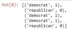 Image by author
text
import sklearn.naive_bayes
text
# Define model
model = sklearn.naive_bayes.MultinomialNB(alpha=1e-7)
# Train model with votes dataset
model.fit(feature_Train, labels_Train)
 Image by author
Evaluate Model Performance
With the model computed, let us now evaluate the performance. We get a quick overview of the model's effectiveness by printing the first 10 rows of the result:
text
predicted_party = model.predict(feature_vecs[:10])
party_probabilities = model.predict_proba(feature_vecs[:10])
text
results = pandas.DataFrame({
        'party': votes['class'][:10],
        'predicted': pandas.Categorical.from_codes(
            predicted_party, votes['class'][:10].cat.categories),
        'proba(Republican)': party_probabilities[:, 0],
        'proba(Democrat)': party_probabilities[:, 1],
    })
results
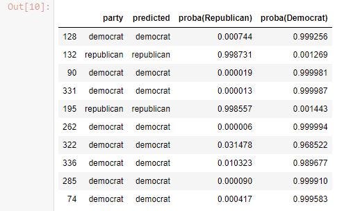 Image by author
As you examine these results notice:
- There is 1 clear classification error, 1 classification that is undecided, and 8 cases correctly classified.
- In most cases, the probability of the class predicted (score) is much larger than for the other class, including for the cases with classification errors.
- One case has nearly identical probabilities for the classes.
As a next step, we compute the confusion matrix and performance metrics for this model:
text
import sklearn.metrics
text
def confusion_matrix(labels, predicted_labels, label_classes):
    return pandas.DataFrame(
        sklearn.metrics.confusion_matrix(labels, predicted_labels),
        index=[label_classes],
        columns=label_classes)
text
def performance(results):
    accuracy = sklearn.metrics.accuracy_score(
        results['party'].cat.codes, results['predicted'].cat.codes)
    precision = sklearn.metrics.precision_score(
            results['party'].cat.codes, results['predicted'].cat.codes)
    recall = sklearn.metrics.recall_score(
            results['party'].cat.codes, results['predicted'].cat.codes)
text
print('Accuracy = %.3f, Precision = %.3f, Recall = %.3f' % (accuracy, precision, recall))

    return confusion_matrix(
        results['party'],
        results['predicted'],
        results.party.cat.categories)
text
performance(results)
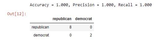 Image by author
The results are reasonably good looking at only the first 10 of 435 congresspeople.
Execute the code in the cell below to compute and print an evaluation of the model using all the data and compare the results to the first model:
text
predicted_party = model.predict(feature_vecs)
party_probabilities = model.predict_proba(feature_vecs)
text
results_all = pandas.DataFrame({
        'party': votes['class'],
        'predicted': pandas.Categorical.from_codes(
            predicted_party, votes['class'].cat.categories),
        'proba(democrat)': party_probabilities[:, 0],
        'proba(republican)': party_probabilities[:, 1],
    })
performance(results_all)
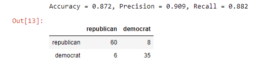 Image by author
Laplace Smoothing
The Laplace smoothing method is an effective way to deal with data sets that do not have sufficient samples to compute probabilities. This method avoids the case where 𝑝(𝑥𝑗|𝐶𝑘)=0p(xj|Ck)=0.
The code in the cell below computes a naive Bayes model using the same congressional vote data, but with a Laplace smoother with a span of 3 data points. Execute this code and examine the results:
text
predicted_party = model.predict(feature_vecs)
party_probabilities = model.predict_proba(feature_vecs)
text
results_all = pandas.DataFrame({
        'party': votes['class'],
        'predicted': pandas.Categorical.from_codes(
            predicted_party, votes['class'].cat.categories),
        'proba(democrat)': party_probabilities[:, 0],
        'proba(republican)': party_probabilities[:, 1],
    })
performance(results_all)
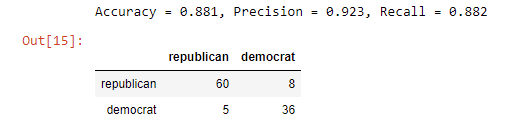 Image by author
The results are similar to the model computed without Laplace smoothing. This result is expected as all the cases in the data set have sufficient data.
Another Example - Census Income
Now we can try another binary classification example. The code in the cell below loads some sample US Census data. We want to build and evaluate a naive Bayes model to classify people by high and low income using $50,000 as the cut-off. Execute this code and examine the features in the data set.
text
# income is a pd read_csv function from a source URL that no longer works
income.head()
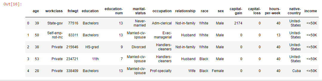 Image by author
text
income.shape
 Image by author
text
income.info()
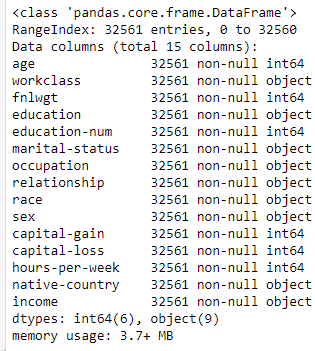 Image by author
text
income.describe()
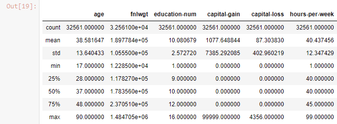 Image by author
Reducing Features
We can see some features which are likely to be collinear. There is also one feature, fnlwgtwhich is not useful in classifying these people. The code in the cell below removes these columns. Execute this code to create a data set with reduced features:
text
income = income.drop(['workclass', 'fnlwgt', 'education-num', 'relationship'], axis=1)
income.head(10)
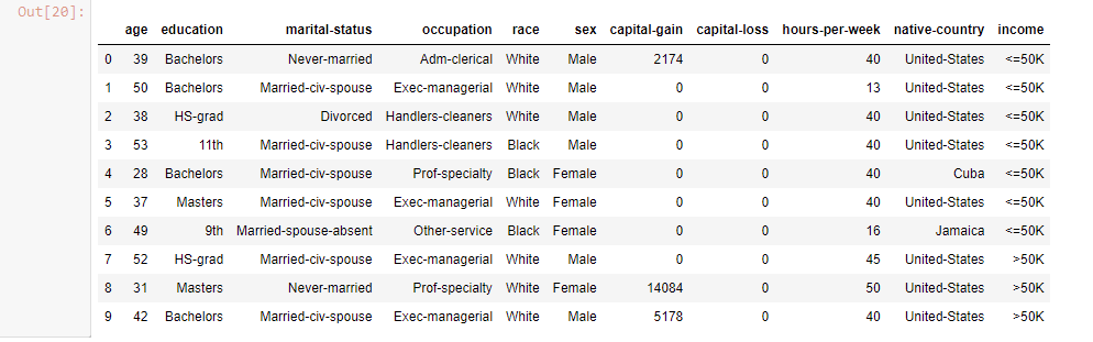 Image by author
Now I compute a Naive Bayes model to classify
income using the features in the Income data set:
text
for c in income.columns:
    if income[c].dtype == 'object':
        income[c] = income[c].astype('category')
text
income_label_col = 'income'
text
income_labels = income[income_label_col].cat.codes
text
features = []
for c in income.columns:
    if c != income_label_col:
        if str(income[c].dtype) == 'category':
            features.append(income[c].cat.codes)
        else:
            features.append(income[c])
income_feature_vecs = numpy.array(features).T
text
# Create model
model = sklearn.naive_bayes.MultinomialNB(alpha=3)
model.fit(income_feature_vecs, income_labels)
 Image by author
text
features[8]
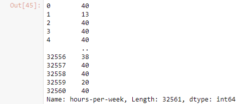 Image by author
text
conditional_probas = pandas.DataFrame(model.feature_log_prob_, columns=income.columns[:-1])
conditional_probas
 Image by author
text
(-conditional_probas).plot(kind='bar')
pyplot.show()
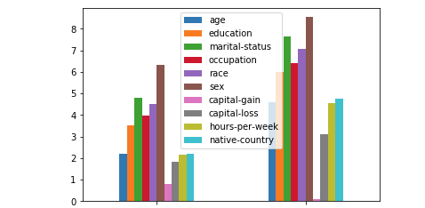 Image by author
Changing Number of Features
Let us now investigate the effect of adding more data samples to the naive Bayes model. The code in the cell below computes and evaluates naive Bayes models using 2, 3, 4, 5, and 6 votes. Execute this code and compare the results to those obtained using the full data set:
text
label_col = 'class'
text
# We need to convert our categorical values to numeric feature vectors
feature_vecs = numpy.array([
        votes[c].cat.codes
        for c in votes.columns
        if c != label_col]).T
print(feature_vecs.shape)
text
# we also need to convert our label (democrat vs republican) to numeric values
labels = votes[label_col].cat.codes
# take a look at the mapping for the first 5 values like so
list(zip(votes[label_col][:5], labels[:5]))
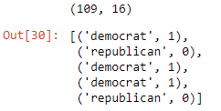 Image by author
text
for num_features in [2, 3, 4, 5, 6]:
    model = sklearn.naive_bayes.MultinomialNB()
    model.fit(feature_vecs[:, :num_features], labels)
text
predicted_votes = model.predict(feature_vecs[:, :num_features])
text
print('Number of features = %d' % num_features)
    accuracy = sklearn.metrics.accuracy_score(labels, predicted_votes)
    precision = sklearn.metrics.precision_score(labels, predicted_votes)
    recall = sklearn.metrics.recall_score(labels, predicted_votes)
    print('Accuracy = %.3f, Precision = %.3f, Recall = %.3f' % (accuracy, precision, recall))
    print('Confusion matrix:')
    print(confusion_matrix(labels, predicted_votes, votes['class'].cat.categories))
    print('')
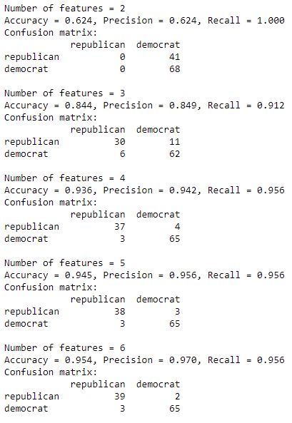 Image by author
You can see from these results, that the model gains accuracy rapidly with just a few features. In fact, 5 or 6 of the 16 features provide equivalent results.
Compute a Naive Bayes model, compute and print the performance statistics for 100, 500, 1000, 2000, 8000, and 32561 rows of the
incomedata set:
text
NumberOfRowsTests = [100, 500, 1000, 2000, 8000, 32561]
for num_rows in (NumberOfRowsTests):
    model = sklearn.naive_bayes.MultinomialNB()
    model.fit(income_feature_vecs[:num_rows, :], income_labels[:num_rows])
text
predicted_income = model.predict(income_feature_vecs[:num_rows, :])
    income_probabilities = model.predict_proba(income_feature_vecs[:num_rows, :])

    accuracy = sklearn.metrics.accuracy_score(income_labels[:num_rows], predicted_income)
    precision = sklearn.metrics.precision_score(income_labels[:num_rows], predicted_income)
    recall = sklearn.metrics.recall_score(income_labels[:num_rows], predicted_income)
    print('%6.0f rows:  Accuracy = %.3f, Precision = %.3f, Recall = %.3f' % (num_rows, accuracy, precision, recall))
    print('Confusion matrix:')
    print(confusion_matrix(
            income_labels[:num_rows], predicted_income, income.income.cat.categories), 'n')
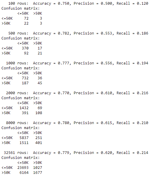 Image by author
Summary
In this notebook I have worked through the following:
- Theory of Naive Bayes models
- Pitfalls of Naive Bayes
- Good regularization properties
- Computationally efficiency
- Examples of computing and evaluating Naive Bayes models
- Examine the effects of data set size on the results of Naive Bayes models
- An explanation of Supervised Learning
Remember that while Naive Bayes is a useful and powerful classifier - this model should always be compared against a logistic regression model. This heuristic allows for a useful sanity check and it provides an important ground truth for evaluating your model.
I hope you have enjoyed this article! Whether you are new to the concept or simply are in need of a refresher I want my readers to have a deep, and complete intuition and understanding of these complex yet highly important topics in data science and machine learning.
Please subscribe if you want me to continue writing on similar topics!
Find me on Linkedin
Physicist cum Data Scientist- Available for new opportunity | SaaS | Sports | Start-ups | Scale-ups
Register Now to Continue Reading
Unlock Towards Data Science with a Free Account
All articles on Towards Data Science are available to registered users. Create a free account today to access this article and thousands more.
Register for freeSign in to your account
 Written By
See all from James Andrew Godwin
Deep DivesMachine LearningNaive BayesPythonSupervised Learning
Share This Article
Towards Data Science is a community publication. Submit your insights to reach our global audience and earn through the TDS Author Payment Program.
Write for TDS
Related Articles
Machine Learning
Hyper-parameter tuning for machine learning models is a trial and error game. To succeed, it is best to avoid the following mistakes.
Georgia Deaconu
January 28, 20224 min read
An example of using FEDOT and other AutoML libraries on real-world data with gaps and non-stationarity
Mikhail Sarafanov
July 2, 202113 min read
Mastering the Art of Python Project Setup: A Step-by-Step Guide
Johannes Schmidt
October 21, 202212 min read
Artificial Intelligence
Convolutional neural networks can help us in performing extremely important classifications for our communications, satellites, people...
Piero Paialunga
December 21, 20206 min read
Deep Learning
Speed up your training, and iterate faster
Michael Clayton
September 19, 202211 min read
Artificial Intelligence
Simply explaining the most common characteristics of Markov Chains
Egor Howell
February 21, 20223 min read
Machine Learning
With the ans
Soner Yıldırım
November 25, 20226 min read
Artificial Intelligence
Discussing theory and implementation with Python and Scikit-learn
Rukshan Pramoditha
May 6, 20239 min read
Data Science
A brief intro to a python package that generates the code while you analyze your data
Roman Orac
May 31, 20223 min read
Your home for data science and AI. The world's leading publication for data science, data analytics, data engineering, machine learning, and artificial intelligence professionals.
Subscribe to Our NewsletterWrite For TDS•About•Advertise•Privacy Policy•Terms of Use
© Insight Media Group, LLC 2026•The New Stack•roadmap.sh•Creator Network
Recommended Articles
Close