{
"source_file": "0930",
"source_platform": "Medium",
"author": "Muhammad Ardi Putra",
"title_listed": "MobileNetV2 Paper Walkthrough: The Smarter Tiny Giant",
"keywords": "",
"domain": "图像处理",
"content_type": "深度技术解析",
"is_paid_flag": "否",
"url": "https://towardsdatascience.com/mobilenetv2-paper-walkthrough-the-smarter-tiny-giant/",
"publish_date": "2025-10-03",
"corpus_stage": "",
"notes": "",
"id": "ea1a58e4f157",
"collected_at": "2026-10-02T02:40:18",
"title": "MobileNetV2 Paper Walkthrough: The Smarter Tiny Giant | Towards Data Science",
"body_markdown": "\nWe value your privacy\nWe use cookies to enhance your browsing experience, serve personalised ads or content, and analyse our traffic. By clicking \"Accept All\", you consent to our use of cookies.\nCustomise Reject All Accept All\nCustomise Consent Preferences \nWe use cookies to help you navigate efficiently and perform certain functions. You will find detailed information about all cookies under each consent category below.\nThe cookies that are categorised as \"Necessary\" are stored on your browser as they are essential for enabling the basic functionalities of the site. ... Show more\nNecessaryAlways Active\nNecessary cookies are required to enable the basic features of this site, such as providing secure log-in or adjusting your consent preferences. These cookies do not store any personally identifiable data.\n * Cookie\nBCTempID\n * Duration\n10 minutes\n * Description\nNo description available.\n\n\n * Cookie\n__cf_bm\n * Duration\n1 hour\n * Description\nThis cookie, set by Cloudflare, is used to support Cloudflare Bot Management. \n\n\n * Cookie\nAWSALBCORS\n * Duration\n7 days\n * Description\nAmazon Web Services set this cookie for load balancing.\n\n\n * Cookie\n_cfuvid\n * Duration\nsession\n * Description\nCloudflare sets this cookie to track users across sessions to optimize user experience by maintaining session consistency and providing personalized services\n\n\n * Cookie\nli_gc\n * Duration\n6 months\n * Description\nLinkedin set this cookie for storing visitor's consent regarding using cookies for non-essential purposes.\n\n\n * Cookie\n__hssrc\n * Duration\nsession\n * Description\nThis cookie is set by Hubspot whenever it changes the session cookie. The __hssrc cookie set to 1 indicates that the user has restarted the browser, and if the cookie does not exist, it is assumed to be a new session.\n\n\n * Cookie\n__hssc\n * Duration\n1 hour\n * Description\nHubSpot sets this cookie to keep track of sessions and to determine if HubSpot should increment the session number and timestamps in the __hstc cookie.\n\n\n * Cookie\nwpEmojiSettingsSupports\n * Duration\nsession\n * Description\nWordPress sets this cookie when a user interacts with emojis on a WordPress site. It helps determine if the user's browser can display emojis properly.\n\n\n * Cookie\nBCSessionID\n * Duration\n1 year 1 month 4 days\n * Description\nBlueconic sets this cookie as a unique identifier for the BlueConic profile.\n\n\n * Cookie\n_octo\n * Duration\n1 year\n * Description\nNo description available.\n\n\n * Cookie\nlogged_in\n * Duration\n1 year\n * Description\nNo description available.\n\n\n * Cookie\n__Secure-YEC\n * Duration\npast\n * Description\nYouTube sets this cookie to stores the user's video player preferences using embedded YouTube video\n\n\n * Cookie\n__eoi\n * Duration\n6 months\n * Description\nDescription is currently not available.\n\n\n * Cookie\nAWSALBTGCORS\n * Duration\n7 days\n * Description\nNo description available.\n\n\n * Cookie\nlogin-status-p\n * Duration\npast\n * Description\nDescription is currently not available.\n\n\n * Cookie\nAWSALBTG\n * Duration\n7 days\n * Description\nNo description available.\n\n\n * Cookie\ncsrf_token\n * Duration\nsession\n * Description\nNo description available.\n\n\n * Cookie\ntoken_v2\n * Duration\n1 day\n * Description\nDescription is currently not available.\n\n\n * Cookie\nD\n * Duration\n1 year\n * Description\nDescription is currently not available.\n\n\n * Cookie\nPHPSESSID\n * Duration\nsession\n * Description\nThis cookie is native to PHP applications. The cookie stores and identifies a user's unique session ID to manage user sessions on the website. The cookie is a session cookie and will be deleted when all the browser windows are closed.\n\n\n * Cookie\nVISITOR_PRIVACY_METADATA\n * Duration\n6 months\n * Description\nYouTube sets this cookie to store the user's cookie consent state for the current domain. \n\n\n * Cookie\ncookietest\n * Duration\nsession\n * Description\nThe cookietest cookie is typically used to determine whether the user's browser accepts cookies, essential for website functionality and user experience.\n\n\n * Cookie\n__Host-airtable-session\n * Duration\n1 year\n * Description\nThis cookie is used to enable us to integrate the services of Airtable.\n\n\n * Cookie\n__Host-airtable-session.sig\n * Duration\n1 year\n * Description\nThis cookie is used to enable us to integrate the services of Airtable.\n\n\n * Cookie\nm\n * Duration\n1 year 1 month 4 days\n * Description\nStripe sets this cookie for fraud prevention purposes. It identifies the device used to access the website, allowing the website to be formatted accordingly.\n\n\n * Cookie\nBIGipServer*\n * Duration\nsession\n * Description\nMarketo sets this cookie to collect information about the user's online activity and build a profile about their interests to provide advertisements relevant to the user. \n\n\n * Cookie\n__cfruid\n * Duration\nsession\n * Description\nCloudflare sets this cookie to identify trusted web traffic.\n\n\n * Cookie\n_GRECAPTCHA\n * Duration\n6 months\n * Description\nGoogle Recaptcha service sets this cookie to identify bots to protect the website against malicious spam attacks.\n\n\n * Cookie\n__Secure-YNID\n * Duration\n6 months\n * Description\nGoogle cookie used to protect user security and prevent fraud, especially during the login process.\n\n\n * Cookie\ncookieyes-consent\n * Duration\n1 year\n * Description\nCookieYes sets this cookie to remember users' consent preferences so that their preferences are respected on subsequent visits to this site. It does not collect or store any personal information about the site visitors.\n\n\nFunctional\nFunctional cookies help perform certain functionalities like sharing the content of the website on social media platforms, collecting feedback, and other third-party features.\n * Cookie\nlidc\n * Duration\n1 day\n * Description\nLinkedIn sets the lidc cookie to facilitate data center selection.\n\n\n * Cookie\nbrw\n * Duration\n1 year\n * Description\nNo description available.\n\n\n * Cookie\nbrwConsent\n * Duration\n5 minutes\n * Description\nDescription is currently not available.\n\n\n * Cookie\nWMF-Uniq\n * Duration\n1 year\n * Description\nDescription is currently not available.\n\n\n * Cookie\nloom_anon_comment\n * Duration\n1 year\n * Description\nNo description available.\n\n\n * Cookie\nloom_referral_video\n * Duration\nsession\n * Description\nDescription is currently not available.\n\n\n * Cookie\nVISITOR_INFO1_LIVE\n * Duration\n6 months\n * Description\nA cookie set by YouTube to measure bandwidth that determines whether the user gets the new or old player interface.\n\n\n * Cookie\nyt-remote-connected-devices\n * Duration\nNever Expires\n * Description\nYouTube sets this cookie to store the user's video preferences using embedded YouTube videos.\n\n\n * Cookie\nytidb::LAST_RESULT_ENTRY_KEY\n * Duration\nNever Expires\n * Description\nThe cookie ytidb::LAST_RESULT_ENTRY_KEY is used by YouTube to store the last search result entry that was clicked by the user. This information is used to improve the user experience by providing more relevant search results in the future.\n\n\n * Cookie\nyt-remote-device-id\n * Duration\nNever Expires\n * Description\nYouTube sets this cookie to store the user's video preferences using embedded YouTube videos.\n\n\n * Cookie\nyt-remote-session-name\n * Duration\nsession\n * Description\nThe yt-remote-session-name cookie is used by YouTube to store the user's video player preferences using embedded YouTube video.\n\n\n * Cookie\nyt-remote-fast-check-period\n * Duration\nsession\n * Description\nThe yt-remote-fast-check-period cookie is used by YouTube to store the user's video player preferences for embedded YouTube videos.\n\n\n * Cookie\nyt-remote-session-app\n * Duration\nsession\n * Description\nThe yt-remote-session-app cookie is used by YouTube to store user preferences and information about the interface of the embedded YouTube video player.\n\n\n * Cookie\nyt-remote-cast-available\n * Duration\nsession\n * Description\nThe yt-remote-cast-available cookie is used to store the user's preferences regarding whether casting is available on their YouTube video player.\n\n\n * Cookie\nyt-remote-cast-installed\n * Duration\nsession\n * Description\nThe yt-remote-cast-installed cookie is used to store the user's video player preferences using embedded YouTube video.\n\n\n * Cookie\ncp_session\n * Duration\n3 months\n * Description\nCodepen sets this cookie for Help systems found in the website.\n\n\n * Cookie\nloid\n * Duration\n1 year 1 month 4 days\n * Description\nThis cookie is set by the Reddit. The cookie enables the sharing of content from the website onto the social media platform.\n\n\nAnalytics\nAnalytical cookies are used to understand how visitors interact with the website. These cookies help provide information on metrics such as the number of visitors, bounce rate, traffic source, etc.\n * Cookie\n__hstc\n * Duration\n6 months\n * Description\nHubspot set this main cookie for tracking visitors. It contains the domain, initial timestamp (first visit), last timestamp (last visit), current timestamp (this visit), and session number (increments for each subsequent session).\n\n\n * Cookie\nhubspotutk\n * Duration\n6 months\n * Description\nHubSpot sets this cookie to keep track of the visitors to the website. This cookie is passed to HubSpot on form submission and used when deduplicating contacts.\n\n\n * Cookie\n_ga\n * Duration\n1 year 1 month 4 days\n * Description\nGoogle Analytics sets this cookie to calculate visitor, session and campaign data and track site usage for the site's analytics report. The cookie stores information anonymously and assigns a randomly generated number to recognise unique visitors.\n\n\n * Cookie\n_ga_*\n * Duration\n1 year 1 month 4 days\n * Description\nGoogle Analytics sets this cookie to store and count page views.\n\n\n * Cookie\n__Host-psifi.analyticsTrace\n * Duration\n6 hours\n * Description\nDescription is currently not available.\n\n\n * Cookie\n__Host-psifi.analyticsTraceV2\n * Duration\n6 hours\n * Description\nDescription is currently not available.\n\n\n * Cookie\n_gh_sess\n * Duration\nsession\n * Description\nGitHub sets this cookie for temporary application and framework state between pages like what step the user is on in a multiple step form.\n\n\n * Cookie\nYSC\n * Duration\nsession\n * Description\nYSC cookie is set by Youtube and is used to track the views of embedded videos on Youtube pages.\n\n\n * Cookie\najs_anonymous_id\n * Duration\n1 year\n * Description\nThis cookie is set by Segment to count the number of people who visit a certain site by tracking if they have visited before.\n\n\n * Cookie\nvuid\n * Duration\n1 year 1 month 4 days\n * Description\nVimeo installs this cookie to collect tracking information by setting a unique ID to embed videos on the website. \n\n\nPerformance\nPerformance cookies are used to understand and analyse the key performance indexes of the website which helps in delivering a better user experience for the visitors.\n * Cookie\nAWSALB\n * Duration\n7 days\n * Description\nAWSALB is an application load balancer cookie set by Amazon Web Services to map the session to the target.\n\n\n * Cookie\nacq\n * Duration\npast\n * Description\nDescription is currently not available.\n\n\n * Cookie\nacq.sig\n * Duration\npast\n * Description\nDescription is currently not available.\n\n\n * Cookie\nptc\n * Duration\n2 years\n * Description\nNo description available.\n\n\nAdvertisement\nAdvertisement cookies are used to provide visitors with customised advertisements based on the pages you visited previously and to analyse the effectiveness of the ad campaigns.\n * Cookie\nmuc_ads\n * Duration\n1 year 1 month 4 days\n * Description\nTwitter sets this cookie to collect user behaviour and interaction data to optimize the website.\n\n\n * Cookie\nguest_id_marketing\n * Duration\n1 year 1 month 4 days\n * Description\nTwitter sets this cookie to identify and track the website visitor.\n\n\n * Cookie\nguest_id_ads\n * Duration\n1 year 1 month 4 days\n * Description\nTwitter sets this cookie to identify and track the website visitor.\n\n\n * Cookie\npersonalization_id\n * Duration\n1 year 1 month 4 days\n * Description\nTwitter sets this cookie to integrate and share features for social media and also store information about how the user uses the website, for tracking and targeting.\n\n\n * Cookie\nguest_id\n * Duration\n1 year 1 month 4 days\n * Description\nTwitter sets this cookie to identify and track the website visitor. It registers if a user is signed in to the Twitter platform and collects information about ad preferences.\n\n\n * Cookie\nbcookie\n * Duration\n1 year\n * Description\nLinkedIn sets this cookie from LinkedIn share buttons and ad tags to recognize browser IDs.\n\n\n * Cookie\n__Secure-ROLLOUT_TOKEN\n * Duration\n6 months\n * Description\nYouTube sets this cookie to manage feature rollout and experimentation. It helps Google control which new features or interface changes are shown to users as part of testing and staged rollouts, ensuring consistent experience for a given user during an experiment.\n\n\n * Cookie\nyt.innertube::nextId\n * Duration\nNever Expires\n * Description\nYouTube sets this cookie to register a unique ID to store data on what videos from YouTube the user has seen.\n\n\n * Cookie\nyt.innertube::requests\n * Duration\nNever Expires\n * Description\nYouTube sets this cookie to register a unique ID to store data on what videos from YouTube the user has seen.\n\n\n * Cookie\nsession_tracker\n * Duration\nsession\n * Description\nThis cookie is set by the Reddit. This cookie is used to identify trusted web traffic. It also helps in adverstising on the website.\n\n\n * Cookie\nedgebucket\n * Duration\nsession\n * Description\nReddit sets this cookie to save the information about a log-on Reddit user, for the purpose of advertisement recommendations and updating the content.\n\n\n * Cookie\ndid\n * Duration\n1 year\n * Description\nArbor sets this cookie to show targeted ads to site visitors.This cookie expires after 2 months or 1 year.\n\n\nUncategorised\nOther uncategorised cookies are those that are being analysed and have not been classified into a category as yet.\nNo cookies to display.\nReject All Save My Preferences Accept All\nToggle Search[](https://towardsdatascience.com/)Toggle Mobile Navigation\n[](https://towardsdatascience.com/)\nPublish AI, ML & data-science insights to a global community of data professionals.\nSign in[Submit an Article](https://write.insightmediagroup.io)\n[Latest](https://towardsdatascience.com/latest/)[Editor's Picks](https://towardsdatascience.com/tag/editors-pick/)[Newsletter](https://towardsdatascience.com/tag/the-variable/)[ShipAI](https://towardsdatascience.com/shipai/)\n* * *\n[Write For TDS](https://towardsdatascience.com/submissions/)\n[LinkedIn](https://www.linkedin.com/company/towards-data-science/)[X](https://x.com/TDataScience)Toggle Search\n[Deep Learning](https://towardsdatascience.com/category/artificial-intelligence/deep-learning/)\n# MobileNetV2 Paper Walkthrough: The Smarter Tiny Giant\nUnderstanding and implementing MobileNetV2 with PyTorch — the next generation of MobileNetV1\n[Muhammad Ardi Putra](https://towardsdatascience.com/author/muhammad_ardi/)\nOctober 3, 202531 min read\n\nPhoto by [Erik Mclean](https://unsplash.com/@introspectivedsgn) on Unsplash\n## Introduction\nMobileNetV1 was a breakthrough in the field of computer vision as it proved that deep learning models do not necessarily need to be computationally expensive to achieve high accuracy. Last month I posted an article where I explained everything about the model as well as its PyTorch implementation from scratch. Check the link at reference number [1] at the end of this article if you are interested in reading it. This first version of MobileNet was first proposed back in April 2017 in a paper titled _MobileNets: Efficient Convolutional Neural Networks for Mobile Vision Applications_[2] by Howard _et al_. from Google. Not long after — in January 2018 to be precise — Sandler _et al_. from the same institution introduced the successor of MobileNetV1 in a paper titled _MobileNetV2: Inverted Residuals and Linear Bottlenecks_ [3], which brings significant improvement over the previous one in terms of both accuracy and efficiency. In this article, I am going to walk you through the ideas proposed in the MobileNetV2 paper and show you how to implement the architecture from scratch.\n···\nLearn this step by step with the interactive [Machine Learning](https://roadmap.sh/machine-learning) roadmap.\n## The Improvements\nThe first version of MobileNet relies solely on the so-called _depthwise separable convolution_ layers. It is indeed necessary to acknowledge that using these layers as a replacement of standard convolutions allows the model to be extremely lightweight. However, authors thought that this architecture could still be improved even further. They came up with an idea where instead of only using depthwise separable convolutions, they also adopted the _inverted residual_ and _linear bottleneck_ mechanisms — which is where the title of the MobileNetV2 paper came from.\n### Inverted Residual\nIf you’re familiar with ResNet, I believe you know the so-called _bottleneck block_. For those who don’t, it is essentially a mechanism where the building block of the network works by following the _wide → narrow → wide_ pattern. Figure 1 below displays the illustration of a bottleneck block used in ResNet. Here we can see that it initially accepts a 256-channel tensor, shrink it to 64, and expands it back to 256.\n\nFigure 1. The building block of ResNet, commonly known as “bottleneck” [4].\nThe inverted version of the above block is commonly known as _inverted bottleneck_ , which follows the _narrow → wide → narrow_ structure. Figure 2 below shows an example from the ConvNeXt paper [5], where the number of channels in the input tensor is 96, expanded to 384, and compressed back to 96 by the last convolution layer. It is important to note that in MobileNetV2 an _inverted bottleneck_ block is called _inverted residual_ for some reasons. So, starting from now on, I will use the term to avoid confusion.\n\nFigure 2. The inverted bottleneck block introduced in ConvNeXt [5].\nAt this point you might be wondering why we don’t just use the standard bottleneck for MobileNetV2. The answer lies in the original purpose of the standard bottleneck design, where it was first introduced to reduce computational complexity. This was essentially done because ResNet is computationally expensive by nature yet rich in information. For this reason, ResNet authors proposed to reduce computational cost by shrinking the tensor size in the middle of each building block, which is how the bottleneck block was born.\nThis reduction in the number of channels does not hurt the model capacity that much since ResNet already has a large number of channels overall. On the other hand, MobileNetV2 is intended to be as lightweight as possible in the first place, which means the model capacity is not as high as ResNet. In order to increase model capacity, authors expand the tensor size in the middle to form the inverted residual block, which allows the model to learn more patterns while only slightly increasing complexity. So in short, the middle part of a bottleneck block (_narrow_) is used for efficiency, while the middle part of an inverted residual block (_wide_) is used to learn complex patterns. If we try to apply a standard bottleneck on MobileNetV2 instead, the computation is going to be even faster, but this might cause a drop in accuracy since the model will lose a significant amount of information.\n### Linear Bottleneck\nThe next concept we need to understand is the so-called _linear bottleneck_. This one is actually pretty simple since what we essentially do here is just to omit the nonlinearity (i.e., the ReLU activation function) in the last layer of each inverted residual block. The use of activation functions in neural networks at the first place is to allow the network to capture complex patterns. However, it will destroy important information instead if we apply it on a low-dimensional tensor, especially in the context of MobileNetV2 where the inverted residual block projects a high dimensional tensor to a smaller one in the last convolution layer. By removing the activation function in the last convolution layer like this, we essentially prevent the model from losing important information. Figure 3 below shows what the inverted residual block used in MobileNetV2 looks like. Notice that ReLU is not applied in the last pointwise convolution, which essentially means that this layer behaves somewhat similarly to a standard linear regression layer. In addition to this figure, the variables _k_ and _k’_ denote the number of input and output channels, respectively. In the intermediate process, we essentially expand the number of channels by _t_ before eventually shrink it to _k’_. I’ll go into more detail on these variables in the next section.\n\nFigure 3. The inverted residual block used in MobileNetV2. Notice that we don’t apply ReLU after the last pointwise convolution layer [3].\n### ReLU6\nSo why do we use ReLU6 instead of regular ReLU? In case you’re not yet familiar with it, this activation function is actually similar to ReLU, except that the output value is capped at 6. So, any input greater than 6 will be mapped to that number. Meanwhile, the behavior for negative inputs is exactly the same. Thus, we can simply say that the output of ReLU6 will always be within the range of 0 to 6 (inclusive). Look at Figure 4 below to better understand this idea.\n\nFigure 4. The ReLU6 activation function [6].\nIn standard ReLU, there is a possibility where the input — and therefore the output — value goes arbitrarily large, in which it potentially causes instability in low-precision environments. Remember that MobileNet is intended to be able to work on small devices, in which we know that such devices typically expect small numbers to save memory, say 8-bit integer. In this particular case, having very large activation values could lead to precision loss or clipping when quantized to low-bit representations. Thus, to keep the values small and within a manageable range, we can simply employ ReLU6 to do so.\n···\n## The Complete MobileNetV2 Architecture\nNow let’s take a look at the complete MobileNetV2 architecture in Figure 5 below. Just like the first version of MobileNet which mostly consists of depthwise separable convolutions, most of the components inside MobileNetV2 are the inverted residual blocks with linear bottlenecks we discussed earlier. Every row in the following table labeled as _bottleneck_ corresponds to a single _stage_ , in which each of them consists of several inverted residual blocks. Talking about the columns in the table, _t_ represents _expansion factor_ used in the middle part of each block, _c_ denotes the number of output channels of each block, _n_ is the number of repeats of the block within that stage, and _s_ indicates the stride of the first block within the stage.\nTo better understand this idea, let’s take a closer look at the stage which the input shape is 56×56×24. Here you can see that the corresponding parameters of this stage are _t_ =6, _c_ =32, _n_ =3, and _s_ =2. This essentially means that the inverted residual stage consists of 3 blocks. All these blocks are identical except that the first one uses stride 2, reducing the spatial dimension by half from 56×56 to 28×28. Next, _c_ =32 is pretty straightforward as it basically says that the number of output channel of each block within the stage is 32. Meanwhile, _t_ =6 indicates that the intermediate layer inside the blocks is 6 times wider than the input, forming the inverted bottleneck structure. So, in this case the number of channels in the process is going to be 32 → 192 → 32. However, it is important to note that the first block within that stage is different, where it uses 24 → 144 → 32 structure thanks to the 24-channel input tensor. If we refer back to Figure 3, these two structures essentially follow the _k → kt → k’_ pattern.\n\nFigure 5. The MobileNetV2 architecture we are about to implement [3].\nIn addition to the above architecture, here we also have skip-connections placed within the inverted residual blocks. This skip-connection will only be applied whenever the stride of the block is set to 1. This is essentially because the spatial dimension of the image will change whenever we use stride 2, causing the output tensor to have different shape to that of the input. Such a difference in tensor shapes will effectively prevent us from performing element-wise summation between the original flow and the skip-connection. See Figure 6 below for the details. Note that the two illustrations in this figure are basically just the visualization of the table in Figure 3.\n\nFigure 6. We don’t implement skip-connection when the stride is set to 2 (i.e., when the layer performs spatial downsampling) [3].\n### Parameter Tuning\nSimilar to MobileNetV1, MobileNetV2 also has two adjustable parameters called _width multiplier_ and _input resolution_. The former is used to adjust the width of the network, while the latter is for changing the resolution of the input image. The architecture you see in Figure 5 is the base configuration, where we set the width multiplier to 1 and the input resolution to 224×224. With these two parameters, we can tune the model to find a sweet spot that balances accuracy and efficiency based on our needs.\nWe can technically choose arbitrary numbers for the two parameters, but authors already provided several predetermined numbers for their experiments. To the width multiplier, we can use 0.75, 0.5 or 0.35, in which all of them will make the model smaller. For instance, if we use 0.5 then all numbers in column _c_ in Figure 5 will be reduced to half of their defaults. To the input resolution, we can choose either 192×192, 160×160, 128×128 or 96×96 as a replacement for 224×224 if you want to lower the number of operations during inference.\n### Some Experimental Results\nFigure 7 below shows what the experimental results done by the authors look like. Even though MobileNetV1 is considered lightweight already, MobileNetV2 proved that its performance is even better in terms of all metrics compared to its predecessor. However, it is necessary to acknowledge that the base MobileNetV2 is not completely superior to other lightweight models especially when taking into account all aspects at once.\n\nFigure 7. The performance of MobileNetV2 compared to other lightweight models on ImageNet dataset [3].\nIn order to achieve even better accuracy, authors also tried to enlarge the model instead by changing the width multiplier to 1.4 for the 224×224 input resolution, which in the above figure corresponds to the result in the last row. Doing this definitely causes the model complexity as well as the computation time to get higher, but in return it allows the model to obtain the highest accuracy. The results in Figure 8 also show the similar thing, where all MobileNetV2 variants completely outperform the MobileNetV1 counterpart, with the largest MobileNetV2 obtaining the highest accuracy among all models.\n\nFigure 8. More results showing the superiority of MobileNetV2 over the existing models and how input resolution affects accuracy [3].\n···\n## MobileNetV2 Implementation\nEvery time I finished learning something, I always wonder if I really understand what I just learned. In the case of deep learning, I (almost) always try to implement the architecture on my own right after reading the paper just to prove to myself that I understand. And here’s the quote that drives me that way:\n> _What I cannot create, I do not understand._\n> __Richard Feynman__\nThis is essentially the reason why I always include the code implementation of the paper I am explaining in my post.\n···\nWhat an intermezzo that was. — Now let’s get back our focus to MobileNetV2. In this section I am going to show you how we can implement the architecture from scratch. As always, the very first thing we need to do is to import the required modules.\npython\n\n```\n# Codeblock 1\nimport torch\nimport torch.nn as nn\nfrom torchinfo import summary\n```\n\nNext, we also need to initialize some configuration variables so that we can easily rescale our model if we want to. The two variables I want to highlight in the Codeblock 2 below are the `WIDTH_MULTIPLIER` and `IMAGE_SIZE`, where these two essentially correspond to the _width multiplier_ and _input resolution_ parameters we discussed earlier. Here I set the two to 1.0 and 224 because I want to implement the base MobileNetV2 architecture.\npython\n\n```\n# Codeblock 2\nBATCH_SIZE = 1\nIMAGE_SIZE = 224\nIN_CHANNELS = 3\nNUM_CLASSES = 1000\nWIDTH_MULTIPLIER = 1.0\n```\n\nIf we take a look at the architectural details in Figure 5, we can see that the rows labeled as _bottleneck_ is a group of blocks, which we previously refer to as _stage_. Meanwhile, each row labeled as _conv2d_ is basically just a standard convolution layer. I’ll start with the latter first because that one is easier to implement.\n### The Standard Convolution Layer\nTalking about the rows labeled with _conv2d_ , you might be asking why we really need to wrap this single convolution layer in a separate class. Can’t we just directly use `nn.Conv2d` in the main class? — In fact, it is mentioned in the paper that every conv layer is always followed by a batch normalization layer before eventually being processed by the ReLU6 activation function. This is actually in accordance with MobileNetV1, where it uses the _conv-BN-ReLU_ structure. In order to make the code cleaner, we can just wrap these layers within a single class so that we don’t necessarily need to define all of them repeatedly. Take a look at the Codeblock 3 below to see how I create the `Conv` class.\npython\n\n```\n# Codeblock 3\nclass Conv(nn.Module):\n def __init__(self, first=False): #(1)\n super().__init__()\n \n if first:\n in_channels = 3 #(2)\n out_channels = int(32*WIDTH_MULTIPLIER) #(3)\n kernel_size = 3 #(4)\n stride = 2 #(5)\n padding = 1 #(6)\n else:\n in_channels = int(320*WIDTH_MULTIPLIER) #(7)\n out_channels = int(1280*WIDTH_MULTIPLIER) #(8)\n kernel_size = 1 #(9)\n stride = 1 #(10)\n padding = 0 #(11)\n \n self.conv = nn.Conv2d(in_channels=in_channels, #(12)\n out_channels=out_channels, \n kernel_size=kernel_size,\n stride=stride, \n padding=padding, \n bias=False)\n self.bn = nn.BatchNorm2d(num_features=out_channels) #(13)\n self.relu6 = nn.ReLU6() #(14)\n \n def forward(self, x):\n x = self.relu6(self.bn(self.conv(x))) #(15)\n return x\n```\n\nEvery time we want to instantiate a `Conv` instance, we need to pass a value for the `first` parameter as shown at the line marked with `#(1)` in the above code. If you take a look at the architecture, you will notice that this `Conv` layer will be used either before the sequence of inverted residuals or right after the sequence. The Figure 9 below displays the architecture again with the two convolutions highlighted in pink and green, respectively. Later in the main class, if we want to instantiate the pink layer, we can simply set the `first` flag to `True`, and if we want to instantiate the green one, we can run it without passing any arguments since I’ve set the flag to `False` by default.\n\nFigure 9. The **Conv** class will be used to instantiate these two convolution layers [3][6].\nUsing a flag like this helps us to apply different configurations for the two convolutions. When we use `first=True`, we set the convolution layer to accept 3 input channels (`#(2)`) and produce a 32-channel tensor (`#(3)`). The kernel size used will be 3×3 (`#(4)`) with a stride of 2 (`#(5)`), effectively downsampling the spatial dimension by half. With this kernel size, we need to set the padding to 1 (`#(6)`) to prevent the convolution process from reducing the spatial dimension even further. All these configurations are essentially taken from the conv layer highlighted in pink.\nMeanwhile, when we use `first=False`, this convolution layer will take a tensor of 320 channels for the input (`#(7)`) and produce another one having 1280 channels (`#(8)`). This green-highlighted layer is a pointwise convolution, hence we need to set the kernel size to 1 (`#(9)`). Since here we won’t perform spatial downsampling, the stride parameter must be set to 1 as shown at line `#(10)` (notice that the input size of this layer and the next one are both 7×7 spatially). Lastly, we set the padding to 0 (`#(11)`) because by nature a 1×1 kernel cannot reduce spatial dimensions on its own.\nAs the parameters for the convolution layer have been defined, the next thing we do in the `Conv` class above is to initialize the convolution layer itself using `nn.Conv2d` (`#(12)`) as well as the batch normalization layer (`#(13)`) and the ReLU6 activation function (`#(14)`). Lastly, we assemble these layers to form the _conv-BN-ReLU_ structure in the `forward()` method (`#(15)`). In addition to the above code, don’t forget to apply `WIDTH_MULTIPLIER` when specifying the number of input and output channels, i.e., at line `#(3)`, `#(7)`, and `#(8)`, so that we can adjust the model size simply by changing the value of the variable.\nNow let’s check if we have implemented the `Conv` class correctly by running the two test cases below. The one in Codeblock 4 demonstrates the pink layer while the Codeblock 5 shows the green one. The shape of the dummy tensor `x` used in both tests are set according to the input shapes required by each of the two layers. Based on the resulting outputs, we can confirm that our implementation is correct since the output tensor shapes match exactly with the expected input shapes of the corresponding subsequent layers.\npython\n\n```\n# Codeblock 4\nconv = Conv(first=True)\nx = torch.randn(1, 3, 224, 224)\n\nout = conv(x)\nout.shape\n```\n\nhttp\n\n```\n# Codeblock 4 Output\ntorch.Size([1, 32, 112, 112])\n```\n\npython\n\n```\n# Codeblock 5\nconv = Conv(first=False)\nx = torch.randn(1, int(320*WIDTH_MULTIPLIER), 7, 7)\n\nout = conv(x)\nout.shape\n```\n\nhttp\n\n```\n# Codeblock 5 Output\ntorch.Size([1, 1280, 7, 7])\n```\n\n···\n### Inverted Residual Block for Stride 2\nAs we have completed the class for standard convolution layers, we will now talk about the one for the inverted residual blocks. Keep in mind that there are cases where we use either stride 1 or 2, which results in a slight difference in the block structure (see Figure 6). In this case I decided to implement them in two separate classes. In terms of practicality, it might indeed be cleaner if we just put them within the same class. However, for the sake of this tutorial I feel like breaking them down into two will make things easier to follow. I am going to implement the one with stride 2 first since this one is simpler thanks to the absence of the skip-connection. See the `InvResidualS2` class in Codeblock 6 below for the details.\npython\n\n```\n# Codeblock 6\nclass InvResidualS2(nn.Module):\n def __init__(self, in_channels, out_channels, t): #(1)\n super().__init__()\n \n in_channels = int(in_channels*WIDTH_MULTIPLIER) #(2)\n out_channels = int(out_channels*WIDTH_MULTIPLIER) #(3)\n \n self.pwconv0 = nn.Conv2d(in_channels=in_channels, #(4)\n out_channels=in_channels*t,\n kernel_size=1, \n stride=1, \n bias=False)\n \n self.bn_pwconv0 = nn.BatchNorm2d(num_features=in_channels*t)\n \n self.dwconv = nn.Conv2d(in_channels=in_channels*t, #(5)\n out_channels=in_channels*t, \n kernel_size=3, #(6)\n stride=2, \n padding=1,\n groups=in_channels*t, #(7)\n bias=False)\n \n self.bn_dwconv = nn.BatchNorm2d(num_features=in_channels*t)\n \n self.pwconv1 = nn.Conv2d(in_channels=in_channels*t, #(8)\n out_channels=out_channels, \n kernel_size=1, \n stride=1, \n bias=False)\n \n self.bn_pwconv1 = nn.BatchNorm2d(num_features=out_channels)\n \n self.relu6 = nn.ReLU6()\n \n def forward(self, x):\n print('original\\t\\t:', x.shape)\n \n x = self.pwconv0(x)\n print('after pwconv0\\t\\t:', x.shape)\n x = self.bn_pwconv0(x)\n print('after bn0_pwconv0\\t:', x.shape)\n x = self.relu6(x)\n print('after relu\\t\\t:', x.shape)\n \n x = self.dwconv(x)\n print('after dwconv\\t\\t:', x.shape)\n x = self.bn_dwconv(x)\n print('after bn_dwconv\\t\\t:', x.shape)\n x = self.relu6(x)\n print('after relu\\t\\t:', x.shape)\n \n x = self.pwconv1(x)\n print('after pwconv1\\t\\t:', x.shape)\n x = self.bn_pwconv1(x)\n print('after bn_pwconv1\\t:', x.shape)\n \n return x\n```\n\nThe above class takes three parameters in order to work: `in_channels`, `out_channels`, and `t`, as written at line `#(1)`. The first two corresponds to the number of input and output channels of the inverted residual block, whereas `t` is the expansion factor for determining the channel count of the _wide_ part of the block. So, what we basically do here is just to make the middle tensors to have `t` times more channels than the input. The number of input and output channels themselves are adjustable via the `WIDTH_MULTIPLIER` variable we initialized earlier as shown at line `#(2)` and `#(3)`.\nWhat we need to do next is to initialize the layers within the inverted residual block according to the structure in Figure 3 and 6. Notice in the two figures that we have a depthwise convolution layer placed between two pointwise convolutions. The first pointwise convolution (`#(4)`) is used to expand the channel dimension from `in_channels` to `in_channels*t`. Subsequently, the depthwise convolution at line `#(5)` is responsible to capture information along the spatial dimension. Here we set the kernel size to 3×3 (`#(6)`), which allows the layer to capture spatial information from its neighboring pixels. Don’t forget to set the `groups` parameter to be the same as the number of input channels to this layer (`#(7)`) since we want the convolution operation to be performed independently of each channel. Next, we process the resulting tensor with the second pointwise convolution (`#(8)`), in which this layer is used to project the tensor to the expected number of output channels of the block.\nIn the `forward()` method, we place the layers one after another. Remember that we use the _conv-BN-ReLU_ structure except for the last convolution, following the convention of linear bottleneck we discussed earlier. Additionally, here I also print out the output shape after each layer so that you can clearly see how the tensor transforms during the process.\nNext, we are going to test whether the `InvResidualS2` class works properly. The following testing code simulates the first inverted residual block (_n=1_) of the third row in the architecture (i.e., the one having 16×112×112 input shape).\npython\n\n```\n# Codeblock 7\ninv_residual_s2 = InvResidualS2(in_channels=16, out_channels=24, t=6)\nx = torch.randn(1, int(16*WIDTH_MULTIPLIER), 112, 112)\n\nout = inv_residual_s2(x)\n```\n\nYou can see at the line marked with `#(1)` in the following output that the first pointwise convolution successfully expands the channel axis from 16 to 96. The spatial dimension shrinks from 112×112 to 56×56 after the tensor being processed by the depthwise convolution layer in the middle (`#(2)`). Lastly, our second pointwise convolution compresses the number of channels to 24 as written at line `#(3)`. This final tensor dimension is now ready to be passed through the next inverted residual block within the same stage.\nhttp\n\n```\n# Codeblock 7 Output\noriginal : torch.Size([1, 16, 112, 112])\nafter pwconv0 : torch.Size([1, 96, 112, 112]) #(1)\nafter bn0_pwconv0 : torch.Size([1, 96, 112, 112])\nafter relu : torch.Size([1, 96, 112, 112])\nafter dwconv : torch.Size([1, 96, 56, 56]) #(2)\nafter bn_dwconv : torch.Size([1, 96, 56, 56])\nafter relu : torch.Size([1, 96, 56, 56])\nafter pwconv1 : torch.Size([1, 24, 56, 56]) #(3)\nafter bn_pwconv1 : torch.Size([1, 24, 56, 56])\n```\n\n···\n### Inverted Residual Block for Stride 1\nThe code used for implementing the inverted residual block with stride 1 is mostly similar to the one with stride 2. See the `InvResidualS1` class in Codeblock 8 below.\npython\n\n```\n# Codeblock 8\nclass InvResidualS1(nn.Module):\n def __init__(self, in_channels, out_channels, t):\n super().__init__()\n \n in_channels = int(in_channels*WIDTH_MULTIPLIER) #(1)\n out_channels = int(out_channels*WIDTH_MULTIPLIER) #(2)\n \n self.in_channels = in_channels\n self.out_channels = out_channels\n \n self.pwconv0 = nn.Conv2d(in_channels=in_channels, \n out_channels=in_channels*t, \n kernel_size=1, \n stride=1, \n bias=False)\n \n self.bn_pwconv0 = nn.BatchNorm2d(num_features=in_channels*t)\n \n self.dwconv = nn.Conv2d(in_channels=in_channels*t, \n out_channels=in_channels*t, \n kernel_size=3, \n stride=1, #(3)\n padding=1,\n groups=in_channels*t, \n bias=False)\n \n self.bn_dwconv = nn.BatchNorm2d(num_features=in_channels*t)\n \n self.pwconv1 = nn.Conv2d(in_channels=in_channels*t, \n out_channels=out_channels, \n kernel_size=1, \n stride=1, \n bias=False)\n \n self.bn_pwconv1 = nn.BatchNorm2d(num_features=out_channels)\n \n self.relu6 = nn.ReLU6()\n \n def forward(self, x):\n \n if self.in_channels == self.out_channels: #(4)\n residual = x #(5)\n print(f'residual\\t\\t: {residual.size()}')\n \n x = self.pwconv0(x)\n print('after pwconv0\\t\\t:', x.shape)\n x = self.bn_pwconv0(x)\n print('after bn_pwconv0\\t:', x.shape)\n x = self.relu6(x)\n print('after relu\\t\\t:', x.shape)\n \n x = self.dwconv(x)\n print('after dwconv\\t\\t:', x.shape)\n x = self.bn_dwconv(x)\n print('after bn_dwconv\\t\\t:', x.shape)\n x = self.relu6(x)\n print('after relu\\t\\t:', x.shape)\n \n x = self.pwconv1(x)\n print('after pwconv1\\t\\t:', x.shape)\n x = self.bn_pwconv1(x)\n print('after bn_pwconv1\\t:', x.shape)\n \n if self.in_channels == self.out_channels:\n x = x + residual #(6)\n print('after summation\\t\\t:', x.shape)\n \n return x\n```\n\nThe first difference we have here is definitely the `stride` parameter itself, especially the one belongs to the depthwise convolution layer at line `#(3)`. By setting the `stride` parameter to 1 like this, the spatial output dimension of this inverted residual block is going to be the same as the input.\nAnother thing that we didn’t do previously is creating instance attributes for `in_channels` and `out_channels` as shown at lines `#(1)` and `#(2)`. We do this now because later on we will need to access these values from the `forward()` method. This is actually just a basic OOP concept, where if we don’t assign them to `self`, then they will only exist locally within the `__init__()` method and won’t be available to other methods in the class.\nInside the `forward()` method itself, what we need to do first is to check whether the number of input and output channels are the same (`#(4)`). If so, we will keep the original input tensor (`#(5)`) to implement the skip-connection, in which this tensor will be element-wise summed with the one from the main flow (`#(6)`). This tensor dimensionality checking is performed because we need to ensure that the two tensors to be summed have the exact same size. We indeed have guaranteed the spatial dimension to remain unchanged since we have set all the three convolution layers to use stride 1. However, there is still a possibility that the number of output channels differs from the input, just like the first block within the stages highlighted in purple, blue and orange in Figure 10 below. In such cases, skip-connection will not be applied because it’s just impossible to perform element-wise summation on tensors with different shapes.\n\nFigure 10. Despite not performing spatial downsampling, there is no skip-connection within the first block in the three highlighted stages since the number of input and output channels are different [3][6].\nNow let’s test the `InvResidualS1` class by running the Codeblock 9 below. Here I am going to simulate the second inverted residual block (_n_ =2) of the third row in the architecture, in which this is actually just the continuation of the previous test case. Here you can see that the dummy tensor we use has the exact same shape as the one we obtained from Codeblock 7, i.e., 24×56×56.\npython\n\n```\n# Codeblock 9\ninv_residual_s1 = InvResidualS1(in_channels=24, out_channels=24, t=6)\nx = torch.randn(1, int(24*WIDTH_MULTIPLIER), 56, 56)\n\nout = inv_residual_s1(x)\n```\n\nAnd below is what the resulting output looks like. It is clearly seen here that the network indeed follows the _narrow → wide → narrow_ structure, which in this case is 24 → 144 → 24. In addition to this, since the spatial dimensions of the input and the output tensors are the same, we can technically stack this inverted residual block as many times as we want.\nhttp\n\n```\n# Codeblock 9 Output\nresidual : torch.Size([1, 24, 56, 56])\nafter pwconv0 : torch.Size([1, 144, 56, 56])\nafter bn_pwconv0 : torch.Size([1, 144, 56, 56])\nafter relu : torch.Size([1, 144, 56, 56])\nafter dwconv : torch.Size([1, 144, 56, 56])\nafter bn_dwconv : torch.Size([1, 144, 56, 56])\nafter relu : torch.Size([1, 144, 56, 56])\nafter pwconv1 : torch.Size([1, 24, 56, 56])\nafter bn_pwconv1 : torch.Size([1, 24, 56, 56])\nafter summation : torch.Size([1, 24, 56, 56])\n```\n\n···\n### The Entire MobileNetV2 Architecture\nAs we have completed defining the `Conv`, `InvResidualS2` and `InvResidualS1` classes, we can now assemble them all to construct the entire MobileNetV2 architecture. Look at the Codeblock 10 below to see how I do that.\npython\n\n```\n# Codeblock 10\nclass MobileNetV2(nn.Module):\n def __init__(self):\n super().__init__()\n \n # Input shape: 3x224x224\n self.first_conv = Conv(first=True)\n \n # Input shape: 32x112x112\n self.inv_residual0 = InvResidualS1(in_channels=32, \n out_channels=16, \n t=1)\n \n # Input shape: 16x112x112\n self.inv_residual1 = nn.ModuleList([InvResidualS2(in_channels=16, \n out_channels=24, \n t=6)])\n \n self.inv_residual1.append(InvResidualS1(in_channels=24, \n out_channels=24, \n t=6))\n \n # Input shape: 24x56x56\n self.inv_residual2 = nn.ModuleList([InvResidualS2(in_channels=24, \n out_channels=32, \n t=6)])\n \n for _ in range(2):\n self.inv_residual2.append(InvResidualS1(in_channels=32, \n out_channels=32, \n t=6))\n \n # Input shape: 32x28x28\n self.inv_residual3 = nn.ModuleList([InvResidualS2(in_channels=32, \n out_channels=64, \n t=6)])\n \n for _ in range(3):\n self.inv_residual3.append(InvResidualS1(in_channels=64, \n out_channels=64, \n t=6))\n \n # Input shape: 64x14x14\n self.inv_residual4 = nn.ModuleList([InvResidualS1(in_channels=64, \n out_channels=96, \n t=6)])\n \n for _ in range(2):\n self.inv_residual4.append(InvResidualS1(in_channels=96, \n out_channels=96, \n t=6))\n \n \n # Input shape: 96x14x14\n self.inv_residual5 = nn.ModuleList([InvResidualS2(in_channels=96, \n out_channels=160, \n t=6)])\n \n for _ in range(2):\n self.inv_residual5.append(InvResidualS1(in_channels=160, \n out_channels=160, \n t=6))\n \n # Input shape: 160x7x7\n self.inv_residual6 = InvResidualS1(in_channels=160, \n out_channels=320, \n t=6)\n \n # Input shape: 320x7x7\n self.last_conv = Conv(first=False)\n \n self.avgpool = nn.AdaptiveAvgPool2d(output_size=(1,1)) #(1)\n self.dropout = nn.Dropout(p=0.2) #(2)\n self.fc = nn.Linear(in_features=int(1280*WIDTH_MULTIPLIER), #(3)\n out_features=1000)\n\n def forward(self, x):\n x = self.first_conv(x)\n print(f\"after first_conv\\t: {x.shape}\")\n \n x = self.inv_residual0(x)\n print(f\"after inv_residual0\\t: {x.shape}\")\n \n for i, layer in enumerate(self.inv_residual1):\n x = layer(x)\n print(f\"after inv_residual1 #{i}\\t: {x.shape}\")\n \n for i, layer in enumerate(self.inv_residual2):\n x = layer(x)\n print(f\"after inv_residual2 #{i}\\t: {x.shape}\")\n \n for i, layer in enumerate(self.inv_residual3):\n x = layer(x)\n print(f\"after inv_residual3 #{i}\\t: {x.shape}\")\n \n for i, layer in enumerate(self.inv_residual4):\n x = layer(x)\n print(f\"after inv_residual4 #{i}\\t: {x.shape}\")\n \n for i, layer in enumerate(self.inv_residual5):\n x = layer(x)\n print(f\"after inv_residual5 #{i}\\t: {x.shape}\")\n \n x = self.inv_residual6(x)\n print(f\"after inv_residual6\\t: {x.shape}\")\n \n x = self.last_conv(x)\n print(f\"after last_conv\\t\\t: {x.shape}\")\n \n x = self.avgpool(x)\n print(f\"after avgpool\\t\\t: {x.shape}\")\n \n x = torch.flatten(x, start_dim=1)\n print(f\"after flatten\\t\\t: {x.shape}\")\n \n x = self.dropout(x)\n print(f\"after dropout\\t\\t: {x.shape}\")\n \n x = self.fc(x)\n print(f\"after fc\\t\\t: {x.shape}\")\n \n return x\n```\n\nDespite being quite long, I think the above code is pretty straightforward since what we basically do here is just to place the blocks according to the given architectural details. However, I really want you to pay attention to the number of block repeats within a single stage (_n_) as well as whether or not the first block in a stage performs downsampling (_s_). This is because the architecture doesn’t seem to follow a specific pattern. There is a case where the block is repeated four times, there are other cases where the repeats is done two or three times, and there is even a stage that consists of a single block only. Not only that, it is also unclear under what conditions authors decided to use stride 1 or 2 for the first block in the stage. However, I believe that this final architecture was obtained based on their internal design iterations and experiments that are not discussed in the paper.\nGoing back to the code, after the stages have been initialized, what we need to do next is to initialize the remaining layers, namely an average pooling layer (`#(1)`), a dropout layer (`#(2)`) and a linear layer (`#(3)`) for the classification head. If you go back to the architectural details, you will notice that the final layer should be a pointwise convolution, not a linear layer like this. In fact, in the case when the spatial dimension of the input tensor is 1×1, a pointwise convolution and a linear layer are equivalent. So, it’s basically fine to use either one.\nTo ensure our MobileNetV2 is working properly, we can run the Codeblock 11 below. Here we can see that this class instance runs without any errors. More importantly, the output shape also matches exactly with the architecture specified in the paper. This confirms that our implementation is correct, and thus ready for training — just don’t forget to adjust the output size of the final layer to match the number of classes in your dataset.\npython\n\n```\n# Codeblock 11\nmobilenetv2 = MobileNetV2()\nx = torch.randn(BATCH_SIZE, IN_CHANNELS, IMAGE_SIZE, IMAGE_SIZE)\n\nout = mobilenetv2(x)\n```\n\nhttp\n\n```\n# Codeblock 11 Output\nafter first_conv : torch.Size([1, 32, 112, 112])\nafter inv_residual1 : torch.Size([1, 16, 112, 112])\nafter inv_residual1 #0 : torch.Size([1, 24, 56, 56])\nafter inv_residual1 #1 : torch.Size([1, 24, 56, 56])\nafter inv_residual2 #0 : torch.Size([1, 32, 28, 28])\nafter inv_residual2 #1 : torch.Size([1, 32, 28, 28])\nafter inv_residual2 #2 : torch.Size([1, 32, 28, 28])\nafter inv_residual3 #0 : torch.Size([1, 64, 14, 14])\nafter inv_residual3 #1 : torch.Size([1, 64, 14, 14])\nafter inv_residual3 #2 : torch.Size([1, 64, 14, 14])\nafter inv_residual3 #3 : torch.Size([1, 64, 14, 14])\nafter inv_residual4 #0 : torch.Size([1, 96, 14, 14])\nafter inv_residual4 #1 : torch.Size([1, 96, 14, 14])\nafter inv_residual4 #2 : torch.Size([1, 96, 14, 14])\nafter inv_residual5 #0 : torch.Size([1, 160, 7, 7])\nafter inv_residual5 #1 : torch.Size([1, 160, 7, 7])\nafter inv_residual5 #2 : torch.Size([1, 160, 7, 7])\nafter inv_residual6 : torch.Size([1, 320, 7, 7])\nafter last_conv : torch.Size([1, 1280, 7, 7])\nafter avgpool : torch.Size([1, 1280, 1, 1])\nafter flatten : torch.Size([1, 1280])\nafter dropout : torch.Size([1, 1280])\nafter fc : torch.Size([1, 1000])\n```\n\nAlternatively, it is also possible to test our MobileNetV2 model using the `summary()` function from `torchinfo`, which will also show us the number of parameters contained within each layer. If you scroll down all the way to the end of the output, you’ll see that this model with default _width multiplier_ has 3,505,960 trainable params. This number is different from the one disclosed in the paper, where according to Figure 7 it should be 3.4 million. However, if we go to the official PyTorch documentation [7], it says that the parameter count of this model is 3,504,872, which is very close to our implementation. Let me know in the comments if you know which parts of the code I should change to make this number match exactly with the one from PyTorch.\npython\n\n```\n# Codeblock 12\nmobilenetv2 = MobileNetV2()\nsummary(mobilenetv2, input_size=(BATCH_SIZE, IN_CHANNELS, IMAGE_SIZE, IMAGE_SIZE))\n```\n\nhttp\n\n```\n# Codeblock 12 Output\n==========================================================================================\nLayer (type:depth-idx) Output Shape Param #\n==========================================================================================\nMobileNetV2 [1, 1000] --\n├─Conv: 1-1 [1, 32, 112, 112] --\n│ └─Conv2d: 2-1 [1, 32, 112, 112] 864\n│ └─BatchNorm2d: 2-2 [1, 32, 112, 112] 64\n│ └─ReLU6: 2-3 [1, 32, 112, 112] --\n├─InvResidualS1: 1-2 [1, 16, 112, 112] --\n│ └─Conv2d: 2-4 [1, 32, 112, 112] 1,024\n│ └─BatchNorm2d: 2-5 [1, 32, 112, 112] 64\n│ └─ReLU6: 2-6 [1, 32, 112, 112] --\n│ └─Conv2d: 2-7 [1, 32, 112, 112] 288\n│ └─BatchNorm2d: 2-8 [1, 32, 112, 112] 64\n│ └─ReLU6: 2-9 [1, 32, 112, 112] --\n│ └─Conv2d: 2-10 [1, 16, 112, 112] 512\n│ └─BatchNorm2d: 2-11 [1, 16, 112, 112] 32\n├─ModuleList: 1-3 -- --\n│ └─InvResidualS2: 2-12 [1, 24, 56, 56] --\n│ │ └─Conv2d: 3-1 [1, 96, 112, 112] 1,536\n│ │ └─BatchNorm2d: 3-2 [1, 96, 112, 112] 192\n│ │ └─ReLU6: 3-3 [1, 96, 112, 112] --\n│ │ └─Conv2d: 3-4 [1, 96, 56, 56] 864\n│ │ └─BatchNorm2d: 3-5 [1, 96, 56, 56] 192\n│ │ └─ReLU6: 3-6 [1, 96, 56, 56] --\n│ │ └─Conv2d: 3-7 [1, 24, 56, 56] 2,304\n│ │ └─BatchNorm2d: 3-8 [1, 24, 56, 56] 48\n│ └─InvResidualS1: 2-13 [1, 24, 56, 56] --\n│ │ └─Conv2d: 3-9 [1, 144, 56, 56] 3,456\n│ │ └─BatchNorm2d: 3-10 [1, 144, 56, 56] 288\n│ │ └─ReLU6: 3-11 [1, 144, 56, 56] --\n│ │ └─Conv2d: 3-12 [1, 144, 56, 56] 1,296\n│ │ └─BatchNorm2d: 3-13 [1, 144, 56, 56] 288\n│ │ └─ReLU6: 3-14 [1, 144, 56, 56] --\n│ │ └─Conv2d: 3-15 [1, 24, 56, 56] 3,456\n│ │ └─BatchNorm2d: 3-16 [1, 24, 56, 56] 48\n├─ModuleList: 1-4 -- --\n│ └─InvResidualS2: 2-14 [1, 32, 28, 28] --\n│ │ └─Conv2d: 3-17 [1, 144, 56, 56] 3,456\n│ │ └─BatchNorm2d: 3-18 [1, 144, 56, 56] 288\n│ │ └─ReLU6: 3-19 [1, 144, 56, 56] --\n│ │ └─Conv2d: 3-20 [1, 144, 28, 28] 1,296\n│ │ └─BatchNorm2d: 3-21 [1, 144, 28, 28] 288\n│ │ └─ReLU6: 3-22 [1, 144, 28, 28] --\n│ │ └─Conv2d: 3-23 [1, 32, 28, 28] 4,608\n│ │ └─BatchNorm2d: 3-24 [1, 32, 28, 28] 64\n│ └─InvResidualS1: 2-15 [1, 32, 28, 28] --\n│ │ └─Conv2d: 3-25 [1, 192, 28, 28] 6,144\n│ │ └─BatchNorm2d: 3-26 [1, 192, 28, 28] 384\n│ │ └─ReLU6: 3-27 [1, 192, 28, 28] --\n│ │ └─Conv2d: 3-28 [1, 192, 28, 28] 1,728\n│ │ └─BatchNorm2d: 3-29 [1, 192, 28, 28] 384\n│ │ └─ReLU6: 3-30 [1, 192, 28, 28] --\n│ │ └─Conv2d: 3-31 [1, 32, 28, 28] 6,144\n│ │ └─BatchNorm2d: 3-32 [1, 32, 28, 28] 64\n│ └─InvResidualS1: 2-16 [1, 32, 28, 28] --\n│ │ └─Conv2d: 3-33 [1, 192, 28, 28] 6,144\n│ │ └─BatchNorm2d: 3-34 [1, 192, 28, 28] 384\n│ │ └─ReLU6: 3-35 [1, 192, 28, 28] --\n│ │ └─Conv2d: 3-36 [1, 192, 28, 28] 1,728\n│ │ └─BatchNorm2d: 3-37 [1, 192, 28, 28] 384\n│ │ └─ReLU6: 3-38 [1, 192, 28, 28] --\n│ │ └─Conv2d: 3-39 [1, 32, 28, 28] 6,144\n│ │ └─BatchNorm2d: 3-40 [1, 32, 28, 28] 64\n├─ModuleList: 1-5 -- --\n│ └─InvResidualS2: 2-17 [1, 64, 14, 14] --\n│ │ └─Conv2d: 3-41 [1, 192, 28, 28] 6,144\n│ │ └─BatchNorm2d: 3-42 [1, 192, 28, 28] 384\n│ │ └─ReLU6: 3-43 [1, 192, 28, 28] --\n│ │ └─Conv2d: 3-44 [1, 192, 14, 14] 1,728\n│ │ └─BatchNorm2d: 3-45 [1, 192, 14, 14] 384\n│ │ └─ReLU6: 3-46 [1, 192, 14, 14] --\n│ │ └─Conv2d: 3-47 [1, 64, 14, 14] 12,288\n│ │ └─BatchNorm2d: 3-48 [1, 64, 14, 14] 128\n│ └─InvResidualS1: 2-18 [1, 64, 14, 14] --\n│ │ └─Conv2d: 3-49 [1, 384, 14, 14] 24,576\n│ │ └─BatchNorm2d: 3-50 [1, 384, 14, 14] 768\n│ │ └─ReLU6: 3-51 [1, 384, 14, 14] --\n│ │ └─Conv2d: 3-52 [1, 384, 14, 14] 3,456\n│ │ └─BatchNorm2d: 3-53 [1, 384, 14, 14] 768\n│ │ └─ReLU6: 3-54 [1, 384, 14, 14] --\n│ │ └─Conv2d: 3-55 [1, 64, 14, 14] 24,576\n│ │ └─BatchNorm2d: 3-56 [1, 64, 14, 14] 128\n│ └─InvResidualS1: 2-19 [1, 64, 14, 14] --\n│ │ └─Conv2d: 3-57 [1, 384, 14, 14] 24,576\n│ │ └─BatchNorm2d: 3-58 [1, 384, 14, 14] 768\n│ │ └─ReLU6: 3-59 [1, 384, 14, 14] --\n│ │ └─Conv2d: 3-60 [1, 384, 14, 14] 3,456\n│ │ └─BatchNorm2d: 3-61 [1, 384, 14, 14] 768\n│ │ └─ReLU6: 3-62 [1, 384, 14, 14] --\n│ │ └─Conv2d: 3-63 [1, 64, 14, 14] 24,576\n│ │ └─BatchNorm2d: 3-64 [1, 64, 14, 14] 128\n│ └─InvResidualS1: 2-20 [1, 64, 14, 14] --\n│ │ └─Conv2d: 3-65 [1, 384, 14, 14] 24,576\n│ │ └─BatchNorm2d: 3-66 [1, 384, 14, 14] 768\n│ │ └─ReLU6: 3-67 [1, 384, 14, 14] --\n│ │ └─Conv2d: 3-68 [1, 384, 14, 14] 3,456\n│ │ └─BatchNorm2d: 3-69 [1, 384, 14, 14] 768\n│ │ └─ReLU6: 3-70 [1, 384, 14, 14] --\n│ │ └─Conv2d: 3-71 [1, 64, 14, 14] 24,576\n│ │ └─BatchNorm2d: 3-72 [1, 64, 14, 14] 128\n├─ModuleList: 1-6 -- --\n│ └─InvResidualS1: 2-21 [1, 96, 14, 14] --\n│ │ └─Conv2d: 3-73 [1, 384, 14, 14] 24,576\n│ │ └─BatchNorm2d: 3-74 [1, 384, 14, 14] 768\n│ │ └─ReLU6: 3-75 [1, 384, 14, 14] --\n│ │ └─Conv2d: 3-76 [1, 384, 14, 14] 3,456\n│ │ └─BatchNorm2d: 3-77 [1, 384, 14, 14] 768\n│ │ └─ReLU6: 3-78 [1, 384, 14, 14] --\n│ │ └─Conv2d: 3-79 [1, 96, 14, 14] 36,864\n│ │ └─BatchNorm2d: 3-80 [1, 96, 14, 14] 192\n│ └─InvResidualS1: 2-22 [1, 96, 14, 14] --\n│ │ └─Conv2d: 3-81 [1, 576, 14, 14] 55,296\n│ │ └─BatchNorm2d: 3-82 [1, 576, 14, 14] 1,152\n│ │ └─ReLU6: 3-83 [1, 576, 14, 14] --\n│ │ └─Conv2d: 3-84 [1, 576, 14, 14] 5,184\n│ │ └─BatchNorm2d: 3-85 [1, 576, 14, 14] 1,152\n│ │ └─ReLU6: 3-86 [1, 576, 14, 14] --\n│ │ └─Conv2d: 3-87 [1, 96, 14, 14] 55,296\n│ │ └─BatchNorm2d: 3-88 [1, 96, 14, 14] 192\n│ └─InvResidualS1: 2-23 [1, 96, 14, 14] --\n│ │ └─Conv2d: 3-89 [1, 576, 14, 14] 55,296\n│ │ └─BatchNorm2d: 3-90 [1, 576, 14, 14] 1,152\n│ │ └─ReLU6: 3-91 [1, 576, 14, 14] --\n│ │ └─Conv2d: 3-92 [1, 576, 14, 14] 5,184\n│ │ └─BatchNorm2d: 3-93 [1, 576, 14, 14] 1,152\n│ │ └─ReLU6: 3-94 [1, 576, 14, 14] --\n│ │ └─Conv2d: 3-95 [1, 96, 14, 14] 55,296\n│ │ └─BatchNorm2d: 3-96 [1, 96, 14, 14] 192\n├─ModuleList: 1-7 -- --\n│ └─InvResidualS2: 2-24 [1, 160, 7, 7] --\n│ │ └─Conv2d: 3-97 [1, 576, 14, 14] 55,296\n│ │ └─BatchNorm2d: 3-98 [1, 576, 14, 14] 1,152\n│ │ └─ReLU6: 3-99 [1, 576, 14, 14] --\n│ │ └─Conv2d: 3-100 [1, 576, 7, 7] 5,184\n│ │ └─BatchNorm2d: 3-101 [1, 576, 7, 7] 1,152\n│ │ └─ReLU6: 3-102 [1, 576, 7, 7] --\n│ │ └─Conv2d: 3-103 [1, 160, 7, 7] 92,160\n│ │ └─BatchNorm2d: 3-104 [1, 160, 7, 7] 320\n│ └─InvResidualS1: 2-25 [1, 160, 7, 7] --\n│ │ └─Conv2d: 3-105 [1, 960, 7, 7] 153,600\n│ │ └─BatchNorm2d: 3-106 [1, 960, 7, 7] 1,920\n│ │ └─ReLU6: 3-107 [1, 960, 7, 7] --\n│ │ └─Conv2d: 3-108 [1, 960, 7, 7] 8,640\n│ │ └─BatchNorm2d: 3-109 [1, 960, 7, 7] 1,920\n│ │ └─ReLU6: 3-110 [1, 960, 7, 7] --\n│ │ └─Conv2d: 3-111 [1, 160, 7, 7] 153,600\n│ │ └─BatchNorm2d: 3-112 [1, 160, 7, 7] 320\n│ └─InvResidualS1: 2-26 [1, 160, 7, 7] --\n│ │ └─Conv2d: 3-113 [1, 960, 7, 7] 153,600\n│ │ └─BatchNorm2d: 3-114 [1, 960, 7, 7] 1,920\n│ │ └─ReLU6: 3-115 [1, 960, 7, 7] --\n│ │ └─Conv2d: 3-116 [1, 960, 7, 7] 8,640\n│ │ └─BatchNorm2d: 3-117 [1, 960, 7, 7] 1,920\n│ │ └─ReLU6: 3-118 [1, 960, 7, 7] --\n│ │ └─Conv2d: 3-119 [1, 160, 7, 7] 153,600\n│ │ └─BatchNorm2d: 3-120 [1, 160, 7, 7] 320\n├─InvResidualS1: 1-8 [1, 320, 7, 7] --\n│ └─Conv2d: 2-27 [1, 960, 7, 7] 153,600\n│ └─BatchNorm2d: 2-28 [1, 960, 7, 7] 1,920\n│ └─ReLU6: 2-29 [1, 960, 7, 7] --\n│ └─Conv2d: 2-30 [1, 960, 7, 7] 8,640\n│ └─BatchNorm2d: 2-31 [1, 960, 7, 7] 1,920\n│ └─ReLU6: 2-32 [1, 960, 7, 7] --\n│ └─Conv2d: 2-33 [1, 320, 7, 7] 307,200\n│ └─BatchNorm2d: 2-34 [1, 320, 7, 7] 640\n├─Conv: 1-9 [1, 1280, 7, 7] --\n│ └─Conv2d: 2-35 [1, 1280, 7, 7] 409,600\n│ └─BatchNorm2d: 2-36 [1, 1280, 7, 7] 2,560\n│ └─ReLU6: 2-37 [1, 1280, 7, 7] --\n├─AdaptiveAvgPool2d: 1-10 [1, 1280, 1, 1] --\n├─Dropout: 1-11 [1, 1280] --\n├─Linear: 1-12 [1, 1000] 1,281,000\n==========================================================================================\nTotal params: 3,505,960\nTrainable params: 3,505,960\nNon-trainable params: 0\nTotal mult-adds (Units.MEGABYTES): 313.65\n==========================================================================================\nInput size (MB): 0.60\nForward/backward pass size (MB): 113.28\nParams size (MB): 14.02\nEstimated Total Size (MB): 127.91\n==========================================================================================\n```\n\n···\n## Ending\nAnd that’s pretty much everything about MobileNetV2. I do encourage you to explore this architecture on your own — at least by actually training it on an image classification dataset. Don’t forget to play around with the _width multiplier_ and the _input resolution_ parameters to find the right balance between prediction accuracy and computational efficiency. You can also find the code used in this article in my GitHub repository [8] by the way.\nI hope you learned something new today. Thanks for reading!\n···\n## References\n[1] Muhammad Ardi. MobileNetV1 Paper Walkthrough: The Tiny Giant. Towards Data Science. [Accessed September 25, 2025].\n[2] Andrew G. Howard _et al._ MobileNets: Efficient Convolutional Neural Networks for Mobile Vision Applications. Arxiv. [Accessed April 7, 2025].\n[3] Mark Sandler _et al._ MobileNetV2: Inverted Residuals and Linear Bottlenecks. Arxiv. [Accessed April 12, 2025].\n[4] Kaiming He _et al._ Deep Residual Learning for Image Recognition. Arxiv. [Accessed April 12, 2025].\n[5] Zhuang Liu _et al._ A ConvNet for the 2020s. Arxiv. [Accessed April 12, 2025].\n[6] Image created originally by author.\n[7] mobilenet_v2. PyTorch. [Accessed April 12, 2025].\n[8] MuhammadArdiPutra. The Smarter Tiny Giant — MobileNetV2. GitHub. [medium_articles/The Smarter Tiny Giant — MobileNetV2.ipynb at main · MuhammadArdiPutra/medium_articles](https://github.com/MuhammadArdiPutra/medium_articles/blob/main/The%20Smarter%20Tiny%20Giant%20-%20MobileNetV2.ipynb) [Accessed April 12, 2025].\n## Register Now to Continue Reading\n### Unlock Towards Data Science with a Free Account\nAll articles on Towards Data Science are available to registered users. Create a free account today to access this article and thousands more.\nRegister for freeSign in to your account\n* * *\n\nWritten By\n## [Muhammad Ardi Putra](https://towardsdatascience.com/author/muhammad_ardi/)\nDeep learning storyteller\n[See all from Muhammad Ardi Putra](https://towardsdatascience.com/author/muhammad_ardi/)\n[Deep Dives](https://towardsdatascience.com/tag/deep-dives/)[Artificial Intelligence](https://towardsdatascience.com/tag/artificial-intelligence/)[Computer Vision](https://towardsdatascience.com/tag/computer-vision/)[Machine Learning](https://towardsdatascience.com/tag/machine-learning/)[Neural Network](https://towardsdatascience.com/tag/neural-network/)\nShare This Article\n * [](https://www.facebook.com/sharer/sharer.php?u=https%3A%2F%2Ftowardsdatascience.com%2Fmobilenetv2-paper-walkthrough-the-smarter-tiny-giant%2F&title=MobileNetV2%20Paper%20Walkthrough%3A%20The%20Smarter%20Tiny%C2%A0Giant)\n * [](https://www.linkedin.com/shareArticle?mini=true&url=https%3A%2F%2Ftowardsdatascience.com%2Fmobilenetv2-paper-walkthrough-the-smarter-tiny-giant%2F&title=MobileNetV2%20Paper%20Walkthrough%3A%20The%20Smarter%20Tiny%C2%A0Giant)\n * [](https://x.com/share?url=https%3A%2F%2Ftowardsdatascience.com%2Fmobilenetv2-paper-walkthrough-the-smarter-tiny-giant%2F&text=MobileNetV2%20Paper%20Walkthrough%3A%20The%20Smarter%20Tiny%C2%A0Giant)\n\n\nTowards Data Science is a community publication. Submit your insights to reach our global audience and earn through the TDS Author Payment Program.\n[Write for TDS](https://towardsdatascience.com/submissions/)\n## Related Articles\n * [](https://towardsdatascience.com/album-covers-by-gans-c5c8ef48f50c/)\n## [Album covers by GANs](https://towardsdatascience.com/album-covers-by-gans-c5c8ef48f50c/)\n[Artificial Intelligence](https://towardsdatascience.com/category/artificial-intelligence/)\nA step-by-step code and intuition guide to generating album covers.\n[Alex Lin](https://towardsdatascience.com/author/alexxlin/)\nJuly 30, 20216 min read\n * [](https://towardsdatascience.com/top-3-non-machine-learning-skills-to-rise-in-kaggle-competitions-d438fec7d551/)\n## [Top 3 non-machine learning skills to rise in Kaggle competitions](https://towardsdatascience.com/top-3-non-machine-learning-skills-to-rise-in-kaggle-competitions-d438fec7d551/)\n[Artificial Intelligence](https://towardsdatascience.com/category/artificial-intelligence/)\nData, creativity, and tactic will make you climb the leaderboard\n[Pranay Dave](https://towardsdatascience.com/author/pranay-dave9/)\nJune 9, 20226 min read\n * [](https://towardsdatascience.com/managing-the-technical-debts-of-machine-learning-systems-5b85d420ab9d/)\n## [Managing the Technical Debts of Machine Learning Systems](https://towardsdatascience.com/managing-the-technical-debts-of-machine-learning-systems-5b85d420ab9d/)\n[Artificial Intelligence](https://towardsdatascience.com/category/artificial-intelligence/)\nExplore the practices with implementation codes for sustainably mitigating the cost of speedy delivery\n[John Leung](https://towardsdatascience.com/author/johnleungtj/)\nSeptember 26, 202310 min read\n * [](https://towardsdatascience.com/do-vision-transformers-see-like-convolutional-neural-networks-paper-explained-91b4bd5185c8/)\n## [Do Vision Transformers See Like Convolutional Neural Networks? (Paper Explained)](https://towardsdatascience.com/do-vision-transformers-see-like-convolutional-neural-networks-paper-explained-91b4bd5185c8/)\n[Deep Learning](https://towardsdatascience.com/category/artificial-intelligence/deep-learning/)\nI will take a closer look at the differences in the obtained representations between CNN and Transformers\n[Akihiro FUJII](https://towardsdatascience.com/author/akichan-f/)\nOctober 9, 202116 min read\n * [](https://towardsdatascience.com/speeding-up-deep-learning-inference-via-unstructured-sparsity-c87e3137cebc/)\n## [Speeding up deep learning inference via unstructured sparsity](https://towardsdatascience.com/speeding-up-deep-learning-inference-via-unstructured-sparsity-c87e3137cebc/)\n[Deep Learning](https://towardsdatascience.com/category/artificial-intelligence/deep-learning/)\nServing large neural networks can be expensive.\n[Ziheng Wang](https://towardsdatascience.com/author/ziheng-4209/)\nSeptember 8, 20205 min read\n * [](https://towardsdatascience.com/forward-and-backward-propagation-of-pooling-layers-in-convolutional-neural-networks-11e36d169bec/)\n## [Forward and Backward propagation of Max Pooling Layer in Convolutional Neural Networks](https://towardsdatascience.com/forward-and-backward-propagation-of-pooling-layers-in-convolutional-neural-networks-11e36d169bec/)\n[Deep Learning](https://towardsdatascience.com/category/artificial-intelligence/deep-learning/)\nTheory and Code\n[Alexey Kravets](https://towardsdatascience.com/author/alexml0123/)\nFebruary 21, 20224 min read\n * [](https://towardsdatascience.com/getting-started-with-pytorch-image-models-timm-a-practitioners-guide-4e77b4bf9055-2/)\n## [Getting Started with PyTorch Image Models (timm): a practitioner's guide](https://towardsdatascience.com/getting-started-with-pytorch-image-models-timm-a-practitioners-guide-4e77b4bf9055-2/)\n[Deep Learning](https://towardsdatascience.com/category/artificial-intelligence/deep-learning/)\nThe purpose of this guide is to explore PyTorch Image Models (timm) from a practitioner's point of view, for use in custom scripts.\n[Chris Hughes](https://towardsdatascience.com/author/chris.p.hughes10/)\nFebruary 1, 202240 min read\n * [](https://towardsdatascience.com/background-removal-with-python-b61671d1508a/)\n## [Background Removal with Python](https://towardsdatascience.com/background-removal-with-python-b61671d1508a/)\n[Data Science](https://towardsdatascience.com/category/data-science/)\nUsing OpenCV to Detect the Foreground\n[Andrew Udell](https://towardsdatascience.com/author/andrew-udell/)\nFebruary 23, 20218 min read\n * [](https://towardsdatascience.com/the-evidence-is-critical-for-classifying-legal-cases-36c1dd6cfd04/)\n## [The Evidence Is Critical for Classifying Legal Cases](https://towardsdatascience.com/the-evidence-is-critical-for-classifying-legal-cases-36c1dd6cfd04/)\n[Artificial Intelligence](https://towardsdatascience.com/category/artificial-intelligence/)\nIdentify the evidence to mine the legal reasoning\n[Vern Walker](https://towardsdatascience.com/author/vern.r.walker/)\nJanuary 19, 20228 min read\n\n\n * [YouTube](https://www.youtube.com/c/TowardsDataScience)\n * [X](https://x.com/TDataScience)\n * [LinkedIn](https://www.linkedin.com/company/towards-data-science/)\n * [Threads](https://www.threads.net/@towardsdatascience)\n * [Bluesky](https://bsky.app/profile/towardsdatascience.com)\n\n\n[](https://towardsdatascience.com/)\nYour home for data science and AI. The world's leading publication for data science, data analytics, data engineering, machine learning, and artificial intelligence professionals.\nSubscribe to Our Newsletter[Write For TDS](https://towardsdatascience.com/submissions/)•[About](https://towardsdatascience.com/about-towards-data-science-d691af11cc2f/)•[Advertise](https://contact.towardsdatascience.com/advertise-with-towards-data-science)•[Privacy Policy](https://towardsdatascience.com/privacy-policy/)•[Terms of Use](https://towardsdatascience.com/website-terms-of-use/)\n© Insight Media Group, LLC 2026•[The New Stack](https://thenewstack.io)•[roadmap.sh](https://roadmap.sh)•[Creator Network](https://insightmediagroup.io/creator-network)\n#### Recommended Articles \nClose\n * [  How Relevance Models Foreshadowed Transformers for NLP ](https://towardsdatascience.com/how-relevance-models-foreshadowed-transformers-for-nlp/ \"How Relevance Models Foreshadowed Transformers for NLP\")\n * [  Javascript Fatigue: HTMX Is All You Need to Build ChatGPT — Part 1 ](https://towardsdatascience.com/javascript-fatigue-you-dont-need-js-to-build-chatgpt/ \"Javascript Fatigue: HTMX Is All You Need to Build ChatGPT — Part 1\")\n * [  The Subset Sum Problem Solved in Linear Time for Dense Enough Inputs ](https://towardsdatascience.com/subset-sum-problem-solved-in-linear-time-for-dense-enough-inputs/ \"The Subset Sum Problem Solved in Linear Time for Dense Enough Inputs\")\n * [  Does Your Company Have a Data Strategy? ](https://towardsdatascience.com/does-your-company-have-a-data-strategy-e8944dbec4ae/ \"Does Your Company Have a Data Strategy?\")\n\n\n",
"metadata": {
"title": "MobileNetV2 Paper Walkthrough: The Smarter Tiny Giant | Towards Data Science",
"description": "Understanding and implementing MobileNetV2 with PyTorch — the next generation of MobileNetV1",
"keywords": null,
"author": "Muhammad Ardi Putra",
"og:locale": "en_US",
"og:type": "article",
"og:title": "MobileNetV2 Paper Walkthrough: The Smarter Tiny Giant",
"og:description": "Understanding and implementing MobileNetV2 with PyTorch — the next generation of MobileNetV1",
"og:url": "https://towardsdatascience.com/mobilenetv2-paper-walkthrough-the-smarter-tiny-giant/",
"og:site_name": "Towards Data Science",
"og:image": "https://assets.insightmediagroup.io/media/wp-content/uploads/2025/10/0_jX-xIvu2lL40B5zA.jpg",
"og:image:width": "1200",
"og:image:height": "800",
"og:image:type": "image/jpeg",
"twitter:card": "summary_large_image",
"twitter:site": "@TDataScience",
"twitter:creator": "@TDataScience",
"twitter:label1": "Written by",
"twitter:data1": "Muhammad Ardi Putra",
"twitter:label2": "Est. reading time",
"twitter:data2": "31 min read",
"article:published_time": "2025-10-03T06:30:01.000Z",
"article:modified_time": "2025-10-03T06:30:01.000Z",
"article:author": "https://towardsdatascience.com/author/muhammad_ardi/"
},
"paywall": {
"listed_paid": false,
"detected": false,
"marker": "",
"public_only": false,
"policy": "付费/会员内容只保留页面公开可见部分,不绕过付费墙"
},
"crawl": {
"success": true,
"status_code": 200,
"error": ""
},
"code_blocks": [
{
"language": "txt",
"file": "attachments/ea1a58e4f157/code/block_000.txt",
"chars": 79
},
{
"language": "txt",
"file": "attachments/ea1a58e4f157/code/block_001.txt",
"chars": 131
},
{
"language": "txt",
"file": "attachments/ea1a58e4f157/code/block_002.txt",
"chars": 1236
},
{
"language": "txt",
"file": "attachments/ea1a58e4f157/code/block_003.txt",
"chars": 95
},
{
"language": "txt",
"file": "attachments/ea1a58e4f157/code/block_004.txt",
"chars": 51
},
{
"language": "txt",
"file": "attachments/ea1a58e4f157/code/block_005.txt",
"chars": 116
},
{
"language": "txt",
"file": "attachments/ea1a58e4f157/code/block_006.txt",
"chars": 49
},
{
"language": "txt",
"file": "attachments/ea1a58e4f157/code/block_007.txt",
"chars": 2216
},
{
"language": "txt",
"file": "attachments/ea1a58e4f157/code/block_008.txt",
"chars": 165
},
{
"language": "txt",
"file": "attachments/ea1a58e4f157/code/block_009.txt",
"chars": 483
},
{
"language": "txt",
"file": "attachments/ea1a58e4f157/code/block_010.txt",
"chars": 2525
},
{
"language": "txt",
"file": "attachments/ea1a58e4f157/code/block_011.txt",
"chars": 163
},
{
"language": "txt",
"file": "attachments/ea1a58e4f157/code/block_012.txt",
"chars": 507
},
{
"language": "txt",
"file": "attachments/ea1a58e4f157/code/block_013.txt",
"chars": 4918
},
{
"language": "txt",
"file": "attachments/ea1a58e4f157/code/block_014.txt",
"chars": 130
},
{
"language": "txt",
"file": "attachments/ea1a58e4f157/code/block_015.txt",
"chars": 1223
},
{
"language": "txt",
"file": "attachments/ea1a58e4f157/code/block_016.txt",
"chars": 126
},
{
"language": "txt",
"file": "attachments/ea1a58e4f157/code/block_017.txt",
"chars": 12947
}
],
"images": [
{
"status": "http_404",
"url": "https://h030.towardsdatascience.com/rest/v2/contentStores/d7d3a4ab-7caf-4383-bbd2-fbf7fb4f1787/items/607686/image?etag=1782161464448&width=500&height=500",
"src": "https://h030.towardsdatascience.com/rest/v2/contentStores/d7d3a4ab-7caf-4383-bbd2-fbf7fb4f1787/items/607686/image?etag=1782161464448&width=500&height=500",
"alt": "",
"downloaded": false,
"discovery": "saved_markdown",
"retried_at": "2026-10-20T18:10:56Z"
},
{
"status": "http_404",
"url": "https://h030.towardsdatascience.com/rest/v2/contentStores/d7d3a4ab-7caf-4383-bbd2-fbf7fb4f1787/items/607639/image?etag=1781250125848&width=500&height=500",
"src": "https://h030.towardsdatascience.com/rest/v2/contentStores/d7d3a4ab-7caf-4383-bbd2-fbf7fb4f1787/items/607639/image?etag=1781250125848&width=500&height=500",
"alt": "",
"downloaded": false,
"discovery": "saved_markdown",
"retried_at": "2026-10-20T18:10:56Z"
},
{
"status": "http_404",
"url": "https://h030.towardsdatascience.com/rest/v2/contentStores/d7d3a4ab-7caf-4383-bbd2-fbf7fb4f1787/items/607930/image?etag=1782124566054&width=500&height=500",
"src": "https://h030.towardsdatascience.com/rest/v2/contentStores/d7d3a4ab-7caf-4383-bbd2-fbf7fb4f1787/items/607930/image?etag=1782124566054&width=500&height=500",
"alt": "",
"downloaded": false,
"discovery": "saved_markdown",
"retried_at": "2026-10-20T18:10:56Z"
},
{
"status": "http_404",
"url": "https://h030.towardsdatascience.com/rest/v2/contentStores/d7d3a4ab-7caf-4383-bbd2-fbf7fb4f1787/items/3660/image?etag=1780176246070&width=500&height=500",
"src": "https://h030.towardsdatascience.com/rest/v2/contentStores/d7d3a4ab-7caf-4383-bbd2-fbf7fb4f1787/items/3660/image?etag=1780176246070&width=500&height=500",
"alt": "",
"downloaded": false,
"discovery": "saved_markdown",
"retried_at": "2026-10-20T18:10:56Z"
}
],
"audio": [],
"videos": [
{
"url": "https://www.youtube.com/c/TowardsDataScience",
"kind": "channel_reference",
"status": "reference_only"
}
],
"links": [
{
"type": "internal",
"href": "https://towardsdatascience.com/"
},
{
"type": "internal",
"href": "https://towardsdatascience.com/latest/"
},
{
"type": "internal",
"href": "https://towardsdatascience.com/tag/editors-pick/"
},
{
"type": "internal",
"href": "https://towardsdatascience.com/tag/the-variable/"
},
{
"type": "internal",
"href": "https://towardsdatascience.com/shipai/"
},
{
"type": "internal",
"href": "https://towardsdatascience.com/submissions/"
},
{
"type": "internal",
"href": "https://towardsdatascience.com/category/artificial-intelligence/deep-learning/"
},
{
"type": "internal",
"href": "https://towardsdatascience.com/author/muhammad_ardi/"
},
{
"type": "internal",
"href": "https://towardsdatascience.com/the-tiny-giant-mobilenetv1/"
},
{
"type": "internal",
"href": "https://towardsdatascience.com/tag/deep-dives/"
},
{
"type": "internal",
"href": "https://towardsdatascience.com/tag/artificial-intelligence/"
},
{
"type": "internal",
"href": "https://towardsdatascience.com/tag/computer-vision/"
},
{
"type": "internal",
"href": "https://towardsdatascience.com/tag/machine-learning/"
},
{
"type": "internal",
"href": "https://towardsdatascience.com/tag/neural-network/"
},
{
"type": "internal",
"href": "https://towardsdatascience.com/album-covers-by-gans-c5c8ef48f50c/"
},
{
"type": "internal",
"href": "https://towardsdatascience.com/category/artificial-intelligence/"
},
{
"type": "internal",
"href": "https://towardsdatascience.com/author/alexxlin/"
},
{
"type": "internal",
"href": "https://towardsdatascience.com/top-3-non-machine-learning-skills-to-rise-in-kaggle-competitions-d438fec7d551/"
},
{
"type": "internal",
"href": "https://towardsdatascience.com/author/pranay-dave9/"
},
{
"type": "internal",
"href": "https://towardsdatascience.com/managing-the-technical-debts-of-machine-learning-systems-5b85d420ab9d/"
},
{
"type": "external",
"href": "https://write.insightmediagroup.io"
},
{
"type": "external",
"href": "https://www.linkedin.com/company/towards-data-science/"
},
{
"type": "external",
"href": "https://x.com/TDataScience"
},
{
"type": "external",
"href": "https://unsplash.com/@introspectivedsgn"
},
{
"type": "external",
"href": "https://roadmap.sh/machine-learning"
},
{
"type": "external",
"href": "https://arxiv.org/abs/1704.04861"
},
{
"type": "external",
"href": "https://arxiv.org/abs/1801.04381"
},
{
"type": "external",
"href": "https://arxiv.org/abs/1512.03385"
},
{
"type": "external",
"href": "https://arxiv.org/abs/2201.03545"
},
{
"type": "external",
"href": "https://pytorch.org/vision/main/models/generated/torchvision.models.mobilenet_v2.html"
},
{
"type": "external",
"href": "https://github.com/MuhammadArdiPutra/medium_articles/blob/main/The%20Smarter%20Tiny%20Giant%20-%20MobileNetV2.ipynb"
},
{
"type": "external",
"href": "https://www.facebook.com/sharer/sharer.php?title=MobileNetV2+Paper+Walkthrough%3A+The+Smarter+Tiny%C2%A0Giant&u=https%3A%2F%2Ftowardsdatascience.com%2Fmobilenetv2-paper-walkthrough-the-smarter-tiny-giant%2F"
},
{
"type": "external",
"href": "https://www.linkedin.com/shareArticle?mini=true&title=MobileNetV2+Paper+Walkthrough%3A+The+Smarter+Tiny%C2%A0Giant&url=https%3A%2F%2Ftowardsdatascience.com%2Fmobilenetv2-paper-walkthrough-the-smarter-tiny-giant%2F"
},
{
"type": "external",
"href": "https://x.com/share?text=MobileNetV2+Paper+Walkthrough%3A+The+Smarter+Tiny%C2%A0Giant&url=https%3A%2F%2Ftowardsdatascience.com%2Fmobilenetv2-paper-walkthrough-the-smarter-tiny-giant%2F"
},
{
"type": "external",
"href": "https://www.youtube.com/c/TowardsDataScience"
},
{
"type": "external",
"href": "https://www.threads.net/@towardsdatascience"
},
{
"type": "external",
"href": "https://bsky.app/profile/towardsdatascience.com"
},
{
"type": "external",
"href": "https://thenewstack.io"
},
{
"type": "external",
"href": "https://roadmap.sh"
},
{
"type": "external",
"href": "https://insightmediagroup.io/creator-network"
}
],
"repair_version": 2,
"repaired_at": "2026-10-20T17:34:50Z",
"source_url": "https://towardsdatascience.com/mobilenetv2-paper-walkthrough-the-smarter-tiny-giant/",
"delivery_status": "unverified",
"discovery_status": "http_403",
"missing_reason": "源页面未重新核验:http_403;已按保留正文补采图片",
"repair_error": "",
"actual_video_files": [],
"expected_saved_body_images": 4,
"image_discovery": "saved_markdown",
"source_body_markdown": "\nWe value your privacy\nWe use cookies to enhance your browsing experience, serve personalised ads or content, and analyse our traffic. By clicking \"Accept All\", you consent to our use of cookies.\nCustomise Reject All Accept All\nCustomise Consent Preferences \nWe use cookies to help you navigate efficiently and perform certain functions. You will find detailed information about all cookies under each consent category below.\nThe cookies that are categorised as \"Necessary\" are stored on your browser as they are essential for enabling the basic functionalities of the site. ... Show more\nNecessaryAlways Active\nNecessary cookies are required to enable the basic features of this site, such as providing secure log-in or adjusting your consent preferences. These cookies do not store any personally identifiable data.\n * Cookie\nBCTempID\n * Duration\n10 minutes\n * Description\nNo description available.\n\n\n * Cookie\n__cf_bm\n * Duration\n1 hour\n * Description\nThis cookie, set by Cloudflare, is used to support Cloudflare Bot Management. \n\n\n * Cookie\nAWSALBCORS\n * Duration\n7 days\n * Description\nAmazon Web Services set this cookie for load balancing.\n\n\n * Cookie\n_cfuvid\n * Duration\nsession\n * Description\nCloudflare sets this cookie to track users across sessions to optimize user experience by maintaining session consistency and providing personalized services\n\n\n * Cookie\nli_gc\n * Duration\n6 months\n * Description\nLinkedin set this cookie for storing visitor's consent regarding using cookies for non-essential purposes.\n\n\n * Cookie\n__hssrc\n * Duration\nsession\n * Description\nThis cookie is set by Hubspot whenever it changes the session cookie. The __hssrc cookie set to 1 indicates that the user has restarted the browser, and if the cookie does not exist, it is assumed to be a new session.\n\n\n * Cookie\n__hssc\n * Duration\n1 hour\n * Description\nHubSpot sets this cookie to keep track of sessions and to determine if HubSpot should increment the session number and timestamps in the __hstc cookie.\n\n\n * Cookie\nwpEmojiSettingsSupports\n * Duration\nsession\n * Description\nWordPress sets this cookie when a user interacts with emojis on a WordPress site. It helps determine if the user's browser can display emojis properly.\n\n\n * Cookie\nBCSessionID\n * Duration\n1 year 1 month 4 days\n * Description\nBlueconic sets this cookie as a unique identifier for the BlueConic profile.\n\n\n * Cookie\n_octo\n * Duration\n1 year\n * Description\nNo description available.\n\n\n * Cookie\nlogged_in\n * Duration\n1 year\n * Description\nNo description available.\n\n\n * Cookie\n__Secure-YEC\n * Duration\npast\n * Description\nYouTube sets this cookie to stores the user's video player preferences using embedded YouTube video\n\n\n * Cookie\n__eoi\n * Duration\n6 months\n * Description\nDescription is currently not available.\n\n\n * Cookie\nAWSALBTGCORS\n * Duration\n7 days\n * Description\nNo description available.\n\n\n * Cookie\nlogin-status-p\n * Duration\npast\n * Description\nDescription is currently not available.\n\n\n * Cookie\nAWSALBTG\n * Duration\n7 days\n * Description\nNo description available.\n\n\n * Cookie\ncsrf_token\n * Duration\nsession\n * Description\nNo description available.\n\n\n * Cookie\ntoken_v2\n * Duration\n1 day\n * Description\nDescription is currently not available.\n\n\n * Cookie\nD\n * Duration\n1 year\n * Description\nDescription is currently not available.\n\n\n * Cookie\nPHPSESSID\n * Duration\nsession\n * Description\nThis cookie is native to PHP applications. The cookie stores and identifies a user's unique session ID to manage user sessions on the website. The cookie is a session cookie and will be deleted when all the browser windows are closed.\n\n\n * Cookie\nVISITOR_PRIVACY_METADATA\n * Duration\n6 months\n * Description\nYouTube sets this cookie to store the user's cookie consent state for the current domain. \n\n\n * Cookie\ncookietest\n * Duration\nsession\n * Description\nThe cookietest cookie is typically used to determine whether the user's browser accepts cookies, essential for website functionality and user experience.\n\n\n * Cookie\n__Host-airtable-session\n * Duration\n1 year\n * Description\nThis cookie is used to enable us to integrate the services of Airtable.\n\n\n * Cookie\n__Host-airtable-session.sig\n * Duration\n1 year\n * Description\nThis cookie is used to enable us to integrate the services of Airtable.\n\n\n * Cookie\nm\n * Duration\n1 year 1 month 4 days\n * Description\nStripe sets this cookie for fraud prevention purposes. It identifies the device used to access the website, allowing the website to be formatted accordingly.\n\n\n * Cookie\nBIGipServer*\n * Duration\nsession\n * Description\nMarketo sets this cookie to collect information about the user's online activity and build a profile about their interests to provide advertisements relevant to the user. \n\n\n * Cookie\n__cfruid\n * Duration\nsession\n * Description\nCloudflare sets this cookie to identify trusted web traffic.\n\n\n * Cookie\n_GRECAPTCHA\n * Duration\n6 months\n * Description\nGoogle Recaptcha service sets this cookie to identify bots to protect the website against malicious spam attacks.\n\n\n * Cookie\n__Secure-YNID\n * Duration\n6 months\n * Description\nGoogle cookie used to protect user security and prevent fraud, especially during the login process.\n\n\n * Cookie\ncookieyes-consent\n * Duration\n1 year\n * Description\nCookieYes sets this cookie to remember users' consent preferences so that their preferences are respected on subsequent visits to this site. It does not collect or store any personal information about the site visitors.\n\n\nFunctional\nFunctional cookies help perform certain functionalities like sharing the content of the website on social media platforms, collecting feedback, and other third-party features.\n * Cookie\nlidc\n * Duration\n1 day\n * Description\nLinkedIn sets the lidc cookie to facilitate data center selection.\n\n\n * Cookie\nbrw\n * Duration\n1 year\n * Description\nNo description available.\n\n\n * Cookie\nbrwConsent\n * Duration\n5 minutes\n * Description\nDescription is currently not available.\n\n\n * Cookie\nWMF-Uniq\n * Duration\n1 year\n * Description\nDescription is currently not available.\n\n\n * Cookie\nloom_anon_comment\n * Duration\n1 year\n * Description\nNo description available.\n\n\n * Cookie\nloom_referral_video\n * Duration\nsession\n * Description\nDescription is currently not available.\n\n\n * Cookie\nVISITOR_INFO1_LIVE\n * Duration\n6 months\n * Description\nA cookie set by YouTube to measure bandwidth that determines whether the user gets the new or old player interface.\n\n\n * Cookie\nyt-remote-connected-devices\n * Duration\nNever Expires\n * Description\nYouTube sets this cookie to store the user's video preferences using embedded YouTube videos.\n\n\n * Cookie\nytidb::LAST_RESULT_ENTRY_KEY\n * Duration\nNever Expires\n * Description\nThe cookie ytidb::LAST_RESULT_ENTRY_KEY is used by YouTube to store the last search result entry that was clicked by the user. This information is used to improve the user experience by providing more relevant search results in the future.\n\n\n * Cookie\nyt-remote-device-id\n * Duration\nNever Expires\n * Description\nYouTube sets this cookie to store the user's video preferences using embedded YouTube videos.\n\n\n * Cookie\nyt-remote-session-name\n * Duration\nsession\n * Description\nThe yt-remote-session-name cookie is used by YouTube to store the user's video player preferences using embedded YouTube video.\n\n\n * Cookie\nyt-remote-fast-check-period\n * Duration\nsession\n * Description\nThe yt-remote-fast-check-period cookie is used by YouTube to store the user's video player preferences for embedded YouTube videos.\n\n\n * Cookie\nyt-remote-session-app\n * Duration\nsession\n * Description\nThe yt-remote-session-app cookie is used by YouTube to store user preferences and information about the interface of the embedded YouTube video player.\n\n\n * Cookie\nyt-remote-cast-available\n * Duration\nsession\n * Description\nThe yt-remote-cast-available cookie is used to store the user's preferences regarding whether casting is available on their YouTube video player.\n\n\n * Cookie\nyt-remote-cast-installed\n * Duration\nsession\n * Description\nThe yt-remote-cast-installed cookie is used to store the user's video player preferences using embedded YouTube video.\n\n\n * Cookie\ncp_session\n * Duration\n3 months\n * Description\nCodepen sets this cookie for Help systems found in the website.\n\n\n * Cookie\nloid\n * Duration\n1 year 1 month 4 days\n * Description\nThis cookie is set by the Reddit. The cookie enables the sharing of content from the website onto the social media platform.\n\n\nAnalytics\nAnalytical cookies are used to understand how visitors interact with the website. These cookies help provide information on metrics such as the number of visitors, bounce rate, traffic source, etc.\n * Cookie\n__hstc\n * Duration\n6 months\n * Description\nHubspot set this main cookie for tracking visitors. It contains the domain, initial timestamp (first visit), last timestamp (last visit), current timestamp (this visit), and session number (increments for each subsequent session).\n\n\n * Cookie\nhubspotutk\n * Duration\n6 months\n * Description\nHubSpot sets this cookie to keep track of the visitors to the website. This cookie is passed to HubSpot on form submission and used when deduplicating contacts.\n\n\n * Cookie\n_ga\n * Duration\n1 year 1 month 4 days\n * Description\nGoogle Analytics sets this cookie to calculate visitor, session and campaign data and track site usage for the site's analytics report. The cookie stores information anonymously and assigns a randomly generated number to recognise unique visitors.\n\n\n * Cookie\n_ga_*\n * Duration\n1 year 1 month 4 days\n * Description\nGoogle Analytics sets this cookie to store and count page views.\n\n\n * Cookie\n__Host-psifi.analyticsTrace\n * Duration\n6 hours\n * Description\nDescription is currently not available.\n\n\n * Cookie\n__Host-psifi.analyticsTraceV2\n * Duration\n6 hours\n * Description\nDescription is currently not available.\n\n\n * Cookie\n_gh_sess\n * Duration\nsession\n * Description\nGitHub sets this cookie for temporary application and framework state between pages like what step the user is on in a multiple step form.\n\n\n * Cookie\nYSC\n * Duration\nsession\n * Description\nYSC cookie is set by Youtube and is used to track the views of embedded videos on Youtube pages.\n\n\n * Cookie\najs_anonymous_id\n * Duration\n1 year\n * Description\nThis cookie is set by Segment to count the number of people who visit a certain site by tracking if they have visited before.\n\n\n * Cookie\nvuid\n * Duration\n1 year 1 month 4 days\n * Description\nVimeo installs this cookie to collect tracking information by setting a unique ID to embed videos on the website. \n\n\nPerformance\nPerformance cookies are used to understand and analyse the key performance indexes of the website which helps in delivering a better user experience for the visitors.\n * Cookie\nAWSALB\n * Duration\n7 days\n * Description\nAWSALB is an application load balancer cookie set by Amazon Web Services to map the session to the target.\n\n\n * Cookie\nacq\n * Duration\npast\n * Description\nDescription is currently not available.\n\n\n * Cookie\nacq.sig\n * Duration\npast\n * Description\nDescription is currently not available.\n\n\n * Cookie\nptc\n * Duration\n2 years\n * Description\nNo description available.\n\n\nAdvertisement\nAdvertisement cookies are used to provide visitors with customised advertisements based on the pages you visited previously and to analyse the effectiveness of the ad campaigns.\n * Cookie\nmuc_ads\n * Duration\n1 year 1 month 4 days\n * Description\nTwitter sets this cookie to collect user behaviour and interaction data to optimize the website.\n\n\n * Cookie\nguest_id_marketing\n * Duration\n1 year 1 month 4 days\n * Description\nTwitter sets this cookie to identify and track the website visitor.\n\n\n * Cookie\nguest_id_ads\n * Duration\n1 year 1 month 4 days\n * Description\nTwitter sets this cookie to identify and track the website visitor.\n\n\n * Cookie\npersonalization_id\n * Duration\n1 year 1 month 4 days\n * Description\nTwitter sets this cookie to integrate and share features for social media and also store information about how the user uses the website, for tracking and targeting.\n\n\n * Cookie\nguest_id\n * Duration\n1 year 1 month 4 days\n * Description\nTwitter sets this cookie to identify and track the website visitor. It registers if a user is signed in to the Twitter platform and collects information about ad preferences.\n\n\n * Cookie\nbcookie\n * Duration\n1 year\n * Description\nLinkedIn sets this cookie from LinkedIn share buttons and ad tags to recognize browser IDs.\n\n\n * Cookie\n__Secure-ROLLOUT_TOKEN\n * Duration\n6 months\n * Description\nYouTube sets this cookie to manage feature rollout and experimentation. It helps Google control which new features or interface changes are shown to users as part of testing and staged rollouts, ensuring consistent experience for a given user during an experiment.\n\n\n * Cookie\nyt.innertube::nextId\n * Duration\nNever Expires\n * Description\nYouTube sets this cookie to register a unique ID to store data on what videos from YouTube the user has seen.\n\n\n * Cookie\nyt.innertube::requests\n * Duration\nNever Expires\n * Description\nYouTube sets this cookie to register a unique ID to store data on what videos from YouTube the user has seen.\n\n\n * Cookie\nsession_tracker\n * Duration\nsession\n * Description\nThis cookie is set by the Reddit. This cookie is used to identify trusted web traffic. It also helps in adverstising on the website.\n\n\n * Cookie\nedgebucket\n * Duration\nsession\n * Description\nReddit sets this cookie to save the information about a log-on Reddit user, for the purpose of advertisement recommendations and updating the content.\n\n\n * Cookie\ndid\n * Duration\n1 year\n * Description\nArbor sets this cookie to show targeted ads to site visitors.This cookie expires after 2 months or 1 year.\n\n\nUncategorised\nOther uncategorised cookies are those that are being analysed and have not been classified into a category as yet.\nNo cookies to display.\nReject All Save My Preferences Accept All\nToggle Search[](https://towardsdatascience.com/)Toggle Mobile Navigation\n[](https://towardsdatascience.com/)\nPublish AI, ML & data-science insights to a global community of data professionals.\nSign in[Submit an Article](https://write.insightmediagroup.io)\n[Latest](https://towardsdatascience.com/latest/)[Editor's Picks](https://towardsdatascience.com/tag/editors-pick/)[Newsletter](https://towardsdatascience.com/tag/the-variable/)[ShipAI](https://towardsdatascience.com/shipai/)\n* * *\n[Write For TDS](https://towardsdatascience.com/submissions/)\n[LinkedIn](https://www.linkedin.com/company/towards-data-science/)[X](https://x.com/TDataScience)Toggle Search\n[Deep Learning](https://towardsdatascience.com/category/artificial-intelligence/deep-learning/)\n# MobileNetV2 Paper Walkthrough: The Smarter Tiny Giant\nUnderstanding and implementing MobileNetV2 with PyTorch — the next generation of MobileNetV1\n[Muhammad Ardi Putra](https://towardsdatascience.com/author/muhammad_ardi/)\nOctober 3, 202531 min read\n\nPhoto by [Erik Mclean](https://unsplash.com/@introspectivedsgn) on Unsplash\n## Introduction\nMobileNetV1 was a breakthrough in the field of computer vision as it proved that deep learning models do not necessarily need to be computationally expensive to achieve high accuracy. Last month I posted an article where I explained everything about the model as well as its PyTorch implementation from scratch. Check the link at reference number [1] at the end of this article if you are interested in reading it. This first version of MobileNet was first proposed back in April 2017 in a paper titled _MobileNets: Efficient Convolutional Neural Networks for Mobile Vision Applications_[2] by Howard _et al_. from Google. Not long after — in January 2018 to be precise — Sandler _et al_. from the same institution introduced the successor of MobileNetV1 in a paper titled _MobileNetV2: Inverted Residuals and Linear Bottlenecks_ [3], which brings significant improvement over the previous one in terms of both accuracy and efficiency. In this article, I am going to walk you through the ideas proposed in the MobileNetV2 paper and show you how to implement the architecture from scratch.\n···\nLearn this step by step with the interactive [Machine Learning](https://roadmap.sh/machine-learning) roadmap.\n## The Improvements\nThe first version of MobileNet relies solely on the so-called _depthwise separable convolution_ layers. It is indeed necessary to acknowledge that using these layers as a replacement of standard convolutions allows the model to be extremely lightweight. However, authors thought that this architecture could still be improved even further. They came up with an idea where instead of only using depthwise separable convolutions, they also adopted the _inverted residual_ and _linear bottleneck_ mechanisms — which is where the title of the MobileNetV2 paper came from.\n### Inverted Residual\nIf you’re familiar with ResNet, I believe you know the so-called _bottleneck block_. For those who don’t, it is essentially a mechanism where the building block of the network works by following the _wide → narrow → wide_ pattern. Figure 1 below displays the illustration of a bottleneck block used in ResNet. Here we can see that it initially accepts a 256-channel tensor, shrink it to 64, and expands it back to 256.\n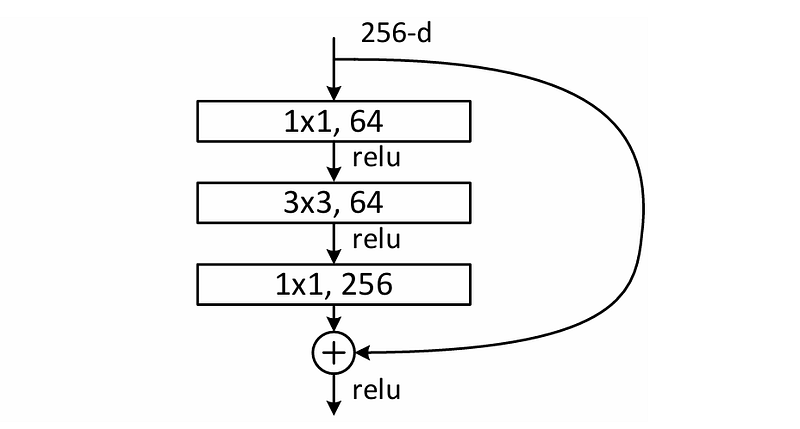\nFigure 1. The building block of ResNet, commonly known as “bottleneck” [4].\nThe inverted version of the above block is commonly known as _inverted bottleneck_ , which follows the _narrow → wide → narrow_ structure. Figure 2 below shows an example from the ConvNeXt paper [5], where the number of channels in the input tensor is 96, expanded to 384, and compressed back to 96 by the last convolution layer. It is important to note that in MobileNetV2 an _inverted bottleneck_ block is called _inverted residual_ for some reasons. So, starting from now on, I will use the term to avoid confusion.\n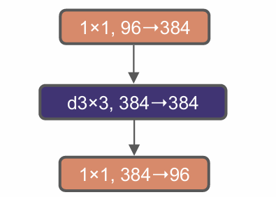\nFigure 2. The inverted bottleneck block introduced in ConvNeXt [5].\nAt this point you might be wondering why we don’t just use the standard bottleneck for MobileNetV2. The answer lies in the original purpose of the standard bottleneck design, where it was first introduced to reduce computational complexity. This was essentially done because ResNet is computationally expensive by nature yet rich in information. For this reason, ResNet authors proposed to reduce computational cost by shrinking the tensor size in the middle of each building block, which is how the bottleneck block was born.\nThis reduction in the number of channels does not hurt the model capacity that much since ResNet already has a large number of channels overall. On the other hand, MobileNetV2 is intended to be as lightweight as possible in the first place, which means the model capacity is not as high as ResNet. In order to increase model capacity, authors expand the tensor size in the middle to form the inverted residual block, which allows the model to learn more patterns while only slightly increasing complexity. So in short, the middle part of a bottleneck block (_narrow_) is used for efficiency, while the middle part of an inverted residual block (_wide_) is used to learn complex patterns. If we try to apply a standard bottleneck on MobileNetV2 instead, the computation is going to be even faster, but this might cause a drop in accuracy since the model will lose a significant amount of information.\n### Linear Bottleneck\nThe next concept we need to understand is the so-called _linear bottleneck_. This one is actually pretty simple since what we essentially do here is just to omit the nonlinearity (i.e., the ReLU activation function) in the last layer of each inverted residual block. The use of activation functions in neural networks at the first place is to allow the network to capture complex patterns. However, it will destroy important information instead if we apply it on a low-dimensional tensor, especially in the context of MobileNetV2 where the inverted residual block projects a high dimensional tensor to a smaller one in the last convolution layer. By removing the activation function in the last convolution layer like this, we essentially prevent the model from losing important information. Figure 3 below shows what the inverted residual block used in MobileNetV2 looks like. Notice that ReLU is not applied in the last pointwise convolution, which essentially means that this layer behaves somewhat similarly to a standard linear regression layer. In addition to this figure, the variables _k_ and _k’_ denote the number of input and output channels, respectively. In the intermediate process, we essentially expand the number of channels by _t_ before eventually shrink it to _k’_. I’ll go into more detail on these variables in the next section.\n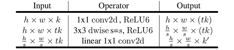\nFigure 3. The inverted residual block used in MobileNetV2. Notice that we don’t apply ReLU after the last pointwise convolution layer [3].\n### ReLU6\nSo why do we use ReLU6 instead of regular ReLU? In case you’re not yet familiar with it, this activation function is actually similar to ReLU, except that the output value is capped at 6. So, any input greater than 6 will be mapped to that number. Meanwhile, the behavior for negative inputs is exactly the same. Thus, we can simply say that the output of ReLU6 will always be within the range of 0 to 6 (inclusive). Look at Figure 4 below to better understand this idea.\n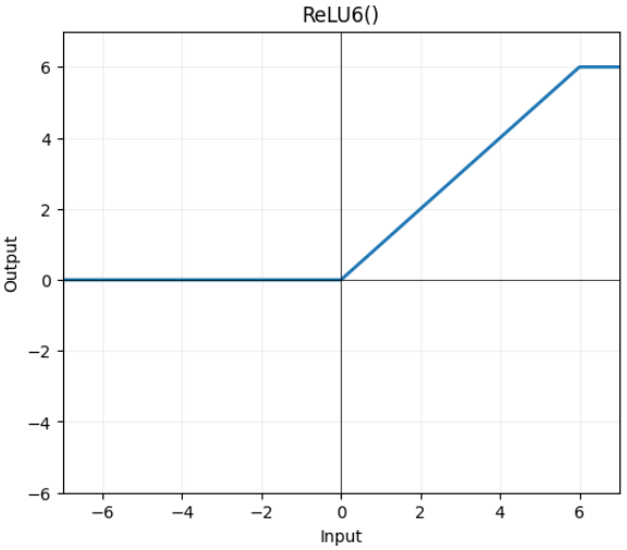\nFigure 4. The ReLU6 activation function [6].\nIn standard ReLU, there is a possibility where the input — and therefore the output — value goes arbitrarily large, in which it potentially causes instability in low-precision environments. Remember that MobileNet is intended to be able to work on small devices, in which we know that such devices typically expect small numbers to save memory, say 8-bit integer. In this particular case, having very large activation values could lead to precision loss or clipping when quantized to low-bit representations. Thus, to keep the values small and within a manageable range, we can simply employ ReLU6 to do so.\n···\n## The Complete MobileNetV2 Architecture\nNow let’s take a look at the complete MobileNetV2 architecture in Figure 5 below. Just like the first version of MobileNet which mostly consists of depthwise separable convolutions, most of the components inside MobileNetV2 are the inverted residual blocks with linear bottlenecks we discussed earlier. Every row in the following table labeled as _bottleneck_ corresponds to a single _stage_ , in which each of them consists of several inverted residual blocks. Talking about the columns in the table, _t_ represents _expansion factor_ used in the middle part of each block, _c_ denotes the number of output channels of each block, _n_ is the number of repeats of the block within that stage, and _s_ indicates the stride of the first block within the stage.\nTo better understand this idea, let’s take a closer look at the stage which the input shape is 56×56×24. Here you can see that the corresponding parameters of this stage are _t_ =6, _c_ =32, _n_ =3, and _s_ =2. This essentially means that the inverted residual stage consists of 3 blocks. All these blocks are identical except that the first one uses stride 2, reducing the spatial dimension by half from 56×56 to 28×28. Next, _c_ =32 is pretty straightforward as it basically says that the number of output channel of each block within the stage is 32. Meanwhile, _t_ =6 indicates that the intermediate layer inside the blocks is 6 times wider than the input, forming the inverted bottleneck structure. So, in this case the number of channels in the process is going to be 32 → 192 → 32. However, it is important to note that the first block within that stage is different, where it uses 24 → 144 → 32 structure thanks to the 24-channel input tensor. If we refer back to Figure 3, these two structures essentially follow the _k → kt → k’_ pattern.\n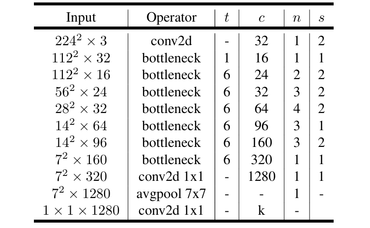\nFigure 5. The MobileNetV2 architecture we are about to implement [3].\nIn addition to the above architecture, here we also have skip-connections placed within the inverted residual blocks. This skip-connection will only be applied whenever the stride of the block is set to 1. This is essentially because the spatial dimension of the image will change whenever we use stride 2, causing the output tensor to have different shape to that of the input. Such a difference in tensor shapes will effectively prevent us from performing element-wise summation between the original flow and the skip-connection. See Figure 6 below for the details. Note that the two illustrations in this figure are basically just the visualization of the table in Figure 3.\n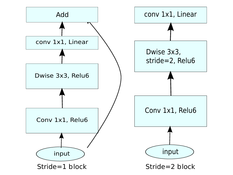\nFigure 6. We don’t implement skip-connection when the stride is set to 2 (i.e., when the layer performs spatial downsampling) [3].\n### Parameter Tuning\nSimilar to MobileNetV1, MobileNetV2 also has two adjustable parameters called _width multiplier_ and _input resolution_. The former is used to adjust the width of the network, while the latter is for changing the resolution of the input image. The architecture you see in Figure 5 is the base configuration, where we set the width multiplier to 1 and the input resolution to 224×224. With these two parameters, we can tune the model to find a sweet spot that balances accuracy and efficiency based on our needs.\nWe can technically choose arbitrary numbers for the two parameters, but authors already provided several predetermined numbers for their experiments. To the width multiplier, we can use 0.75, 0.5 or 0.35, in which all of them will make the model smaller. For instance, if we use 0.5 then all numbers in column _c_ in Figure 5 will be reduced to half of their defaults. To the input resolution, we can choose either 192×192, 160×160, 128×128 or 96×96 as a replacement for 224×224 if you want to lower the number of operations during inference.\n### Some Experimental Results\nFigure 7 below shows what the experimental results done by the authors look like. Even though MobileNetV1 is considered lightweight already, MobileNetV2 proved that its performance is even better in terms of all metrics compared to its predecessor. However, it is necessary to acknowledge that the base MobileNetV2 is not completely superior to other lightweight models especially when taking into account all aspects at once.\n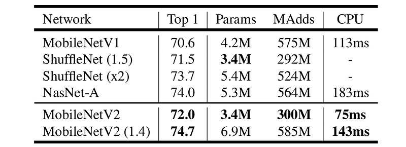\nFigure 7. The performance of MobileNetV2 compared to other lightweight models on ImageNet dataset [3].\nIn order to achieve even better accuracy, authors also tried to enlarge the model instead by changing the width multiplier to 1.4 for the 224×224 input resolution, which in the above figure corresponds to the result in the last row. Doing this definitely causes the model complexity as well as the computation time to get higher, but in return it allows the model to obtain the highest accuracy. The results in Figure 8 also show the similar thing, where all MobileNetV2 variants completely outperform the MobileNetV1 counterpart, with the largest MobileNetV2 obtaining the highest accuracy among all models.\n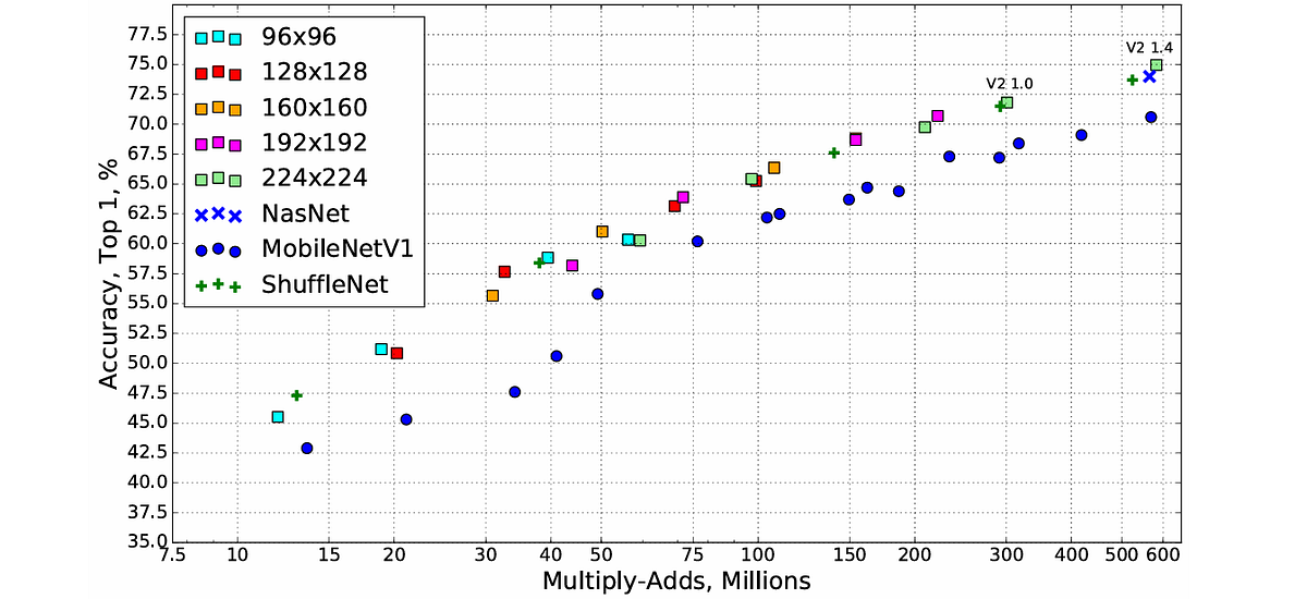\nFigure 8. More results showing the superiority of MobileNetV2 over the existing models and how input resolution affects accuracy [3].\n···\n## MobileNetV2 Implementation\nEvery time I finished learning something, I always wonder if I really understand what I just learned. In the case of deep learning, I (almost) always try to implement the architecture on my own right after reading the paper just to prove to myself that I understand. And here’s the quote that drives me that way:\n> _What I cannot create, I do not understand._\n> __Richard Feynman__\nThis is essentially the reason why I always include the code implementation of the paper I am explaining in my post.\n···\nWhat an intermezzo that was. — Now let’s get back our focus to MobileNetV2. In this section I am going to show you how we can implement the architecture from scratch. As always, the very first thing we need to do is to import the required modules.\npython\n\n```\n# Codeblock 1\nimport torch\nimport torch.nn as nn\nfrom torchinfo import summary\n```\n\nNext, we also need to initialize some configuration variables so that we can easily rescale our model if we want to. The two variables I want to highlight in the Codeblock 2 below are the `WIDTH_MULTIPLIER` and `IMAGE_SIZE`, where these two essentially correspond to the _width multiplier_ and _input resolution_ parameters we discussed earlier. Here I set the two to 1.0 and 224 because I want to implement the base MobileNetV2 architecture.\npython\n\n```\n# Codeblock 2\nBATCH_SIZE = 1\nIMAGE_SIZE = 224\nIN_CHANNELS = 3\nNUM_CLASSES = 1000\nWIDTH_MULTIPLIER = 1.0\n```\n\nIf we take a look at the architectural details in Figure 5, we can see that the rows labeled as _bottleneck_ is a group of blocks, which we previously refer to as _stage_. Meanwhile, each row labeled as _conv2d_ is basically just a standard convolution layer. I’ll start with the latter first because that one is easier to implement.\n### The Standard Convolution Layer\nTalking about the rows labeled with _conv2d_ , you might be asking why we really need to wrap this single convolution layer in a separate class. Can’t we just directly use `nn.Conv2d` in the main class? — In fact, it is mentioned in the paper that every conv layer is always followed by a batch normalization layer before eventually being processed by the ReLU6 activation function. This is actually in accordance with MobileNetV1, where it uses the _conv-BN-ReLU_ structure. In order to make the code cleaner, we can just wrap these layers within a single class so that we don’t necessarily need to define all of them repeatedly. Take a look at the Codeblock 3 below to see how I create the `Conv` class.\npython\n\n```\n# Codeblock 3\nclass Conv(nn.Module):\n def __init__(self, first=False): #(1)\n super().__init__()\n \n if first:\n in_channels = 3 #(2)\n out_channels = int(32*WIDTH_MULTIPLIER) #(3)\n kernel_size = 3 #(4)\n stride = 2 #(5)\n padding = 1 #(6)\n else:\n in_channels = int(320*WIDTH_MULTIPLIER) #(7)\n out_channels = int(1280*WIDTH_MULTIPLIER) #(8)\n kernel_size = 1 #(9)\n stride = 1 #(10)\n padding = 0 #(11)\n \n self.conv = nn.Conv2d(in_channels=in_channels, #(12)\n out_channels=out_channels, \n kernel_size=kernel_size,\n stride=stride, \n padding=padding, \n bias=False)\n self.bn = nn.BatchNorm2d(num_features=out_channels) #(13)\n self.relu6 = nn.ReLU6() #(14)\n \n def forward(self, x):\n x = self.relu6(self.bn(self.conv(x))) #(15)\n return x\n```\n\nEvery time we want to instantiate a `Conv` instance, we need to pass a value for the `first` parameter as shown at the line marked with `#(1)` in the above code. If you take a look at the architecture, you will notice that this `Conv` layer will be used either before the sequence of inverted residuals or right after the sequence. The Figure 9 below displays the architecture again with the two convolutions highlighted in pink and green, respectively. Later in the main class, if we want to instantiate the pink layer, we can simply set the `first` flag to `True`, and if we want to instantiate the green one, we can run it without passing any arguments since I’ve set the flag to `False` by default.\n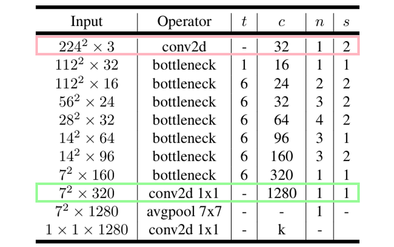\nFigure 9. The **Conv** class will be used to instantiate these two convolution layers [3][6].\nUsing a flag like this helps us to apply different configurations for the two convolutions. When we use `first=True`, we set the convolution layer to accept 3 input channels (`#(2)`) and produce a 32-channel tensor (`#(3)`). The kernel size used will be 3×3 (`#(4)`) with a stride of 2 (`#(5)`), effectively downsampling the spatial dimension by half. With this kernel size, we need to set the padding to 1 (`#(6)`) to prevent the convolution process from reducing the spatial dimension even further. All these configurations are essentially taken from the conv layer highlighted in pink.\nMeanwhile, when we use `first=False`, this convolution layer will take a tensor of 320 channels for the input (`#(7)`) and produce another one having 1280 channels (`#(8)`). This green-highlighted layer is a pointwise convolution, hence we need to set the kernel size to 1 (`#(9)`). Since here we won’t perform spatial downsampling, the stride parameter must be set to 1 as shown at line `#(10)` (notice that the input size of this layer and the next one are both 7×7 spatially). Lastly, we set the padding to 0 (`#(11)`) because by nature a 1×1 kernel cannot reduce spatial dimensions on its own.\nAs the parameters for the convolution layer have been defined, the next thing we do in the `Conv` class above is to initialize the convolution layer itself using `nn.Conv2d` (`#(12)`) as well as the batch normalization layer (`#(13)`) and the ReLU6 activation function (`#(14)`). Lastly, we assemble these layers to form the _conv-BN-ReLU_ structure in the `forward()` method (`#(15)`). In addition to the above code, don’t forget to apply `WIDTH_MULTIPLIER` when specifying the number of input and output channels, i.e., at line `#(3)`, `#(7)`, and `#(8)`, so that we can adjust the model size simply by changing the value of the variable.\nNow let’s check if we have implemented the `Conv` class correctly by running the two test cases below. The one in Codeblock 4 demonstrates the pink layer while the Codeblock 5 shows the green one. The shape of the dummy tensor `x` used in both tests are set according to the input shapes required by each of the two layers. Based on the resulting outputs, we can confirm that our implementation is correct since the output tensor shapes match exactly with the expected input shapes of the corresponding subsequent layers.\npython\n\n```\n# Codeblock 4\nconv = Conv(first=True)\nx = torch.randn(1, 3, 224, 224)\n\nout = conv(x)\nout.shape\n```\n\nhttp\n\n```\n# Codeblock 4 Output\ntorch.Size([1, 32, 112, 112])\n```\n\npython\n\n```\n# Codeblock 5\nconv = Conv(first=False)\nx = torch.randn(1, int(320*WIDTH_MULTIPLIER), 7, 7)\n\nout = conv(x)\nout.shape\n```\n\nhttp\n\n```\n# Codeblock 5 Output\ntorch.Size([1, 1280, 7, 7])\n```\n\n···\n### Inverted Residual Block for Stride 2\nAs we have completed the class for standard convolution layers, we will now talk about the one for the inverted residual blocks. Keep in mind that there are cases where we use either stride 1 or 2, which results in a slight difference in the block structure (see Figure 6). In this case I decided to implement them in two separate classes. In terms of practicality, it might indeed be cleaner if we just put them within the same class. However, for the sake of this tutorial I feel like breaking them down into two will make things easier to follow. I am going to implement the one with stride 2 first since this one is simpler thanks to the absence of the skip-connection. See the `InvResidualS2` class in Codeblock 6 below for the details.\npython\n\n```\n# Codeblock 6\nclass InvResidualS2(nn.Module):\n def __init__(self, in_channels, out_channels, t): #(1)\n super().__init__()\n \n in_channels = int(in_channels*WIDTH_MULTIPLIER) #(2)\n out_channels = int(out_channels*WIDTH_MULTIPLIER) #(3)\n \n self.pwconv0 = nn.Conv2d(in_channels=in_channels, #(4)\n out_channels=in_channels*t,\n kernel_size=1, \n stride=1, \n bias=False)\n \n self.bn_pwconv0 = nn.BatchNorm2d(num_features=in_channels*t)\n \n self.dwconv = nn.Conv2d(in_channels=in_channels*t, #(5)\n out_channels=in_channels*t, \n kernel_size=3, #(6)\n stride=2, \n padding=1,\n groups=in_channels*t, #(7)\n bias=False)\n \n self.bn_dwconv = nn.BatchNorm2d(num_features=in_channels*t)\n \n self.pwconv1 = nn.Conv2d(in_channels=in_channels*t, #(8)\n out_channels=out_channels, \n kernel_size=1, \n stride=1, \n bias=False)\n \n self.bn_pwconv1 = nn.BatchNorm2d(num_features=out_channels)\n \n self.relu6 = nn.ReLU6()\n \n def forward(self, x):\n print('original\\t\\t:', x.shape)\n \n x = self.pwconv0(x)\n print('after pwconv0\\t\\t:', x.shape)\n x = self.bn_pwconv0(x)\n print('after bn0_pwconv0\\t:', x.shape)\n x = self.relu6(x)\n print('after relu\\t\\t:', x.shape)\n \n x = self.dwconv(x)\n print('after dwconv\\t\\t:', x.shape)\n x = self.bn_dwconv(x)\n print('after bn_dwconv\\t\\t:', x.shape)\n x = self.relu6(x)\n print('after relu\\t\\t:', x.shape)\n \n x = self.pwconv1(x)\n print('after pwconv1\\t\\t:', x.shape)\n x = self.bn_pwconv1(x)\n print('after bn_pwconv1\\t:', x.shape)\n \n return x\n```\n\nThe above class takes three parameters in order to work: `in_channels`, `out_channels`, and `t`, as written at line `#(1)`. The first two corresponds to the number of input and output channels of the inverted residual block, whereas `t` is the expansion factor for determining the channel count of the _wide_ part of the block. So, what we basically do here is just to make the middle tensors to have `t` times more channels than the input. The number of input and output channels themselves are adjustable via the `WIDTH_MULTIPLIER` variable we initialized earlier as shown at line `#(2)` and `#(3)`.\nWhat we need to do next is to initialize the layers within the inverted residual block according to the structure in Figure 3 and 6. Notice in the two figures that we have a depthwise convolution layer placed between two pointwise convolutions. The first pointwise convolution (`#(4)`) is used to expand the channel dimension from `in_channels` to `in_channels*t`. Subsequently, the depthwise convolution at line `#(5)` is responsible to capture information along the spatial dimension. Here we set the kernel size to 3×3 (`#(6)`), which allows the layer to capture spatial information from its neighboring pixels. Don’t forget to set the `groups` parameter to be the same as the number of input channels to this layer (`#(7)`) since we want the convolution operation to be performed independently of each channel. Next, we process the resulting tensor with the second pointwise convolution (`#(8)`), in which this layer is used to project the tensor to the expected number of output channels of the block.\nIn the `forward()` method, we place the layers one after another. Remember that we use the _conv-BN-ReLU_ structure except for the last convolution, following the convention of linear bottleneck we discussed earlier. Additionally, here I also print out the output shape after each layer so that you can clearly see how the tensor transforms during the process.\nNext, we are going to test whether the `InvResidualS2` class works properly. The following testing code simulates the first inverted residual block (_n=1_) of the third row in the architecture (i.e., the one having 16×112×112 input shape).\npython\n\n```\n# Codeblock 7\ninv_residual_s2 = InvResidualS2(in_channels=16, out_channels=24, t=6)\nx = torch.randn(1, int(16*WIDTH_MULTIPLIER), 112, 112)\n\nout = inv_residual_s2(x)\n```\n\nYou can see at the line marked with `#(1)` in the following output that the first pointwise convolution successfully expands the channel axis from 16 to 96. The spatial dimension shrinks from 112×112 to 56×56 after the tensor being processed by the depthwise convolution layer in the middle (`#(2)`). Lastly, our second pointwise convolution compresses the number of channels to 24 as written at line `#(3)`. This final tensor dimension is now ready to be passed through the next inverted residual block within the same stage.\nhttp\n\n```\n# Codeblock 7 Output\noriginal : torch.Size([1, 16, 112, 112])\nafter pwconv0 : torch.Size([1, 96, 112, 112]) #(1)\nafter bn0_pwconv0 : torch.Size([1, 96, 112, 112])\nafter relu : torch.Size([1, 96, 112, 112])\nafter dwconv : torch.Size([1, 96, 56, 56]) #(2)\nafter bn_dwconv : torch.Size([1, 96, 56, 56])\nafter relu : torch.Size([1, 96, 56, 56])\nafter pwconv1 : torch.Size([1, 24, 56, 56]) #(3)\nafter bn_pwconv1 : torch.Size([1, 24, 56, 56])\n```\n\n···\n### Inverted Residual Block for Stride 1\nThe code used for implementing the inverted residual block with stride 1 is mostly similar to the one with stride 2. See the `InvResidualS1` class in Codeblock 8 below.\npython\n\n```\n# Codeblock 8\nclass InvResidualS1(nn.Module):\n def __init__(self, in_channels, out_channels, t):\n super().__init__()\n \n in_channels = int(in_channels*WIDTH_MULTIPLIER) #(1)\n out_channels = int(out_channels*WIDTH_MULTIPLIER) #(2)\n \n self.in_channels = in_channels\n self.out_channels = out_channels\n \n self.pwconv0 = nn.Conv2d(in_channels=in_channels, \n out_channels=in_channels*t, \n kernel_size=1, \n stride=1, \n bias=False)\n \n self.bn_pwconv0 = nn.BatchNorm2d(num_features=in_channels*t)\n \n self.dwconv = nn.Conv2d(in_channels=in_channels*t, \n out_channels=in_channels*t, \n kernel_size=3, \n stride=1, #(3)\n padding=1,\n groups=in_channels*t, \n bias=False)\n \n self.bn_dwconv = nn.BatchNorm2d(num_features=in_channels*t)\n \n self.pwconv1 = nn.Conv2d(in_channels=in_channels*t, \n out_channels=out_channels, \n kernel_size=1, \n stride=1, \n bias=False)\n \n self.bn_pwconv1 = nn.BatchNorm2d(num_features=out_channels)\n \n self.relu6 = nn.ReLU6()\n \n def forward(self, x):\n \n if self.in_channels == self.out_channels: #(4)\n residual = x #(5)\n print(f'residual\\t\\t: {residual.size()}')\n \n x = self.pwconv0(x)\n print('after pwconv0\\t\\t:', x.shape)\n x = self.bn_pwconv0(x)\n print('after bn_pwconv0\\t:', x.shape)\n x = self.relu6(x)\n print('after relu\\t\\t:', x.shape)\n \n x = self.dwconv(x)\n print('after dwconv\\t\\t:', x.shape)\n x = self.bn_dwconv(x)\n print('after bn_dwconv\\t\\t:', x.shape)\n x = self.relu6(x)\n print('after relu\\t\\t:', x.shape)\n \n x = self.pwconv1(x)\n print('after pwconv1\\t\\t:', x.shape)\n x = self.bn_pwconv1(x)\n print('after bn_pwconv1\\t:', x.shape)\n \n if self.in_channels == self.out_channels:\n x = x + residual #(6)\n print('after summation\\t\\t:', x.shape)\n \n return x\n```\n\nThe first difference we have here is definitely the `stride` parameter itself, especially the one belongs to the depthwise convolution layer at line `#(3)`. By setting the `stride` parameter to 1 like this, the spatial output dimension of this inverted residual block is going to be the same as the input.\nAnother thing that we didn’t do previously is creating instance attributes for `in_channels` and `out_channels` as shown at lines `#(1)` and `#(2)`. We do this now because later on we will need to access these values from the `forward()` method. This is actually just a basic OOP concept, where if we don’t assign them to `self`, then they will only exist locally within the `__init__()` method and won’t be available to other methods in the class.\nInside the `forward()` method itself, what we need to do first is to check whether the number of input and output channels are the same (`#(4)`). If so, we will keep the original input tensor (`#(5)`) to implement the skip-connection, in which this tensor will be element-wise summed with the one from the main flow (`#(6)`). This tensor dimensionality checking is performed because we need to ensure that the two tensors to be summed have the exact same size. We indeed have guaranteed the spatial dimension to remain unchanged since we have set all the three convolution layers to use stride 1. However, there is still a possibility that the number of output channels differs from the input, just like the first block within the stages highlighted in purple, blue and orange in Figure 10 below. In such cases, skip-connection will not be applied because it’s just impossible to perform element-wise summation on tensors with different shapes.\n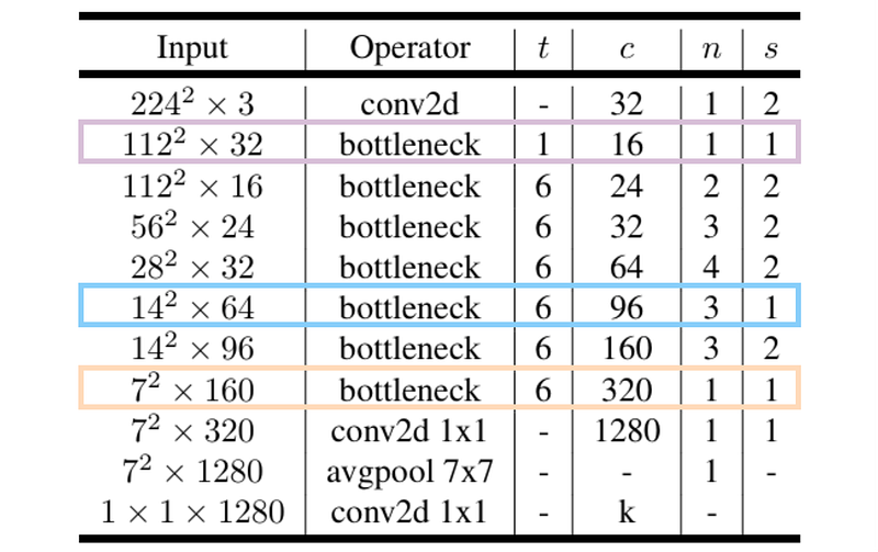\nFigure 10. Despite not performing spatial downsampling, there is no skip-connection within the first block in the three highlighted stages since the number of input and output channels are different [3][6].\nNow let’s test the `InvResidualS1` class by running the Codeblock 9 below. Here I am going to simulate the second inverted residual block (_n_ =2) of the third row in the architecture, in which this is actually just the continuation of the previous test case. Here you can see that the dummy tensor we use has the exact same shape as the one we obtained from Codeblock 7, i.e., 24×56×56.\npython\n\n```\n# Codeblock 9\ninv_residual_s1 = InvResidualS1(in_channels=24, out_channels=24, t=6)\nx = torch.randn(1, int(24*WIDTH_MULTIPLIER), 56, 56)\n\nout = inv_residual_s1(x)\n```\n\nAnd below is what the resulting output looks like. It is clearly seen here that the network indeed follows the _narrow → wide → narrow_ structure, which in this case is 24 → 144 → 24. In addition to this, since the spatial dimensions of the input and the output tensors are the same, we can technically stack this inverted residual block as many times as we want.\nhttp\n\n```\n# Codeblock 9 Output\nresidual : torch.Size([1, 24, 56, 56])\nafter pwconv0 : torch.Size([1, 144, 56, 56])\nafter bn_pwconv0 : torch.Size([1, 144, 56, 56])\nafter relu : torch.Size([1, 144, 56, 56])\nafter dwconv : torch.Size([1, 144, 56, 56])\nafter bn_dwconv : torch.Size([1, 144, 56, 56])\nafter relu : torch.Size([1, 144, 56, 56])\nafter pwconv1 : torch.Size([1, 24, 56, 56])\nafter bn_pwconv1 : torch.Size([1, 24, 56, 56])\nafter summation : torch.Size([1, 24, 56, 56])\n```\n\n···\n### The Entire MobileNetV2 Architecture\nAs we have completed defining the `Conv`, `InvResidualS2` and `InvResidualS1` classes, we can now assemble them all to construct the entire MobileNetV2 architecture. Look at the Codeblock 10 below to see how I do that.\npython\n\n```\n# Codeblock 10\nclass MobileNetV2(nn.Module):\n def __init__(self):\n super().__init__()\n \n # Input shape: 3x224x224\n self.first_conv = Conv(first=True)\n \n # Input shape: 32x112x112\n self.inv_residual0 = InvResidualS1(in_channels=32, \n out_channels=16, \n t=1)\n \n # Input shape: 16x112x112\n self.inv_residual1 = nn.ModuleList([InvResidualS2(in_channels=16, \n out_channels=24, \n t=6)])\n \n self.inv_residual1.append(InvResidualS1(in_channels=24, \n out_channels=24, \n t=6))\n \n # Input shape: 24x56x56\n self.inv_residual2 = nn.ModuleList([InvResidualS2(in_channels=24, \n out_channels=32, \n t=6)])\n \n for _ in range(2):\n self.inv_residual2.append(InvResidualS1(in_channels=32, \n out_channels=32, \n t=6))\n \n # Input shape: 32x28x28\n self.inv_residual3 = nn.ModuleList([InvResidualS2(in_channels=32, \n out_channels=64, \n t=6)])\n \n for _ in range(3):\n self.inv_residual3.append(InvResidualS1(in_channels=64, \n out_channels=64, \n t=6))\n \n # Input shape: 64x14x14\n self.inv_residual4 = nn.ModuleList([InvResidualS1(in_channels=64, \n out_channels=96, \n t=6)])\n \n for _ in range(2):\n self.inv_residual4.append(InvResidualS1(in_channels=96, \n out_channels=96, \n t=6))\n \n \n # Input shape: 96x14x14\n self.inv_residual5 = nn.ModuleList([InvResidualS2(in_channels=96, \n out_channels=160, \n t=6)])\n \n for _ in range(2):\n self.inv_residual5.append(InvResidualS1(in_channels=160, \n out_channels=160, \n t=6))\n \n # Input shape: 160x7x7\n self.inv_residual6 = InvResidualS1(in_channels=160, \n out_channels=320, \n t=6)\n \n # Input shape: 320x7x7\n self.last_conv = Conv(first=False)\n \n self.avgpool = nn.AdaptiveAvgPool2d(output_size=(1,1)) #(1)\n self.dropout = nn.Dropout(p=0.2) #(2)\n self.fc = nn.Linear(in_features=int(1280*WIDTH_MULTIPLIER), #(3)\n out_features=1000)\n\n def forward(self, x):\n x = self.first_conv(x)\n print(f\"after first_conv\\t: {x.shape}\")\n \n x = self.inv_residual0(x)\n print(f\"after inv_residual0\\t: {x.shape}\")\n \n for i, layer in enumerate(self.inv_residual1):\n x = layer(x)\n print(f\"after inv_residual1 #{i}\\t: {x.shape}\")\n \n for i, layer in enumerate(self.inv_residual2):\n x = layer(x)\n print(f\"after inv_residual2 #{i}\\t: {x.shape}\")\n \n for i, layer in enumerate(self.inv_residual3):\n x = layer(x)\n print(f\"after inv_residual3 #{i}\\t: {x.shape}\")\n \n for i, layer in enumerate(self.inv_residual4):\n x = layer(x)\n print(f\"after inv_residual4 #{i}\\t: {x.shape}\")\n \n for i, layer in enumerate(self.inv_residual5):\n x = layer(x)\n print(f\"after inv_residual5 #{i}\\t: {x.shape}\")\n \n x = self.inv_residual6(x)\n print(f\"after inv_residual6\\t: {x.shape}\")\n \n x = self.last_conv(x)\n print(f\"after last_conv\\t\\t: {x.shape}\")\n \n x = self.avgpool(x)\n print(f\"after avgpool\\t\\t: {x.shape}\")\n \n x = torch.flatten(x, start_dim=1)\n print(f\"after flatten\\t\\t: {x.shape}\")\n \n x = self.dropout(x)\n print(f\"after dropout\\t\\t: {x.shape}\")\n \n x = self.fc(x)\n print(f\"after fc\\t\\t: {x.shape}\")\n \n return x\n```\n\nDespite being quite long, I think the above code is pretty straightforward since what we basically do here is just to place the blocks according to the given architectural details. However, I really want you to pay attention to the number of block repeats within a single stage (_n_) as well as whether or not the first block in a stage performs downsampling (_s_). This is because the architecture doesn’t seem to follow a specific pattern. There is a case where the block is repeated four times, there are other cases where the repeats is done two or three times, and there is even a stage that consists of a single block only. Not only that, it is also unclear under what conditions authors decided to use stride 1 or 2 for the first block in the stage. However, I believe that this final architecture was obtained based on their internal design iterations and experiments that are not discussed in the paper.\nGoing back to the code, after the stages have been initialized, what we need to do next is to initialize the remaining layers, namely an average pooling layer (`#(1)`), a dropout layer (`#(2)`) and a linear layer (`#(3)`) for the classification head. If you go back to the architectural details, you will notice that the final layer should be a pointwise convolution, not a linear layer like this. In fact, in the case when the spatial dimension of the input tensor is 1×1, a pointwise convolution and a linear layer are equivalent. So, it’s basically fine to use either one.\nTo ensure our MobileNetV2 is working properly, we can run the Codeblock 11 below. Here we can see that this class instance runs without any errors. More importantly, the output shape also matches exactly with the architecture specified in the paper. This confirms that our implementation is correct, and thus ready for training — just don’t forget to adjust the output size of the final layer to match the number of classes in your dataset.\npython\n\n```\n# Codeblock 11\nmobilenetv2 = MobileNetV2()\nx = torch.randn(BATCH_SIZE, IN_CHANNELS, IMAGE_SIZE, IMAGE_SIZE)\n\nout = mobilenetv2(x)\n```\n\nhttp\n\n```\n# Codeblock 11 Output\nafter first_conv : torch.Size([1, 32, 112, 112])\nafter inv_residual1 : torch.Size([1, 16, 112, 112])\nafter inv_residual1 #0 : torch.Size([1, 24, 56, 56])\nafter inv_residual1 #1 : torch.Size([1, 24, 56, 56])\nafter inv_residual2 #0 : torch.Size([1, 32, 28, 28])\nafter inv_residual2 #1 : torch.Size([1, 32, 28, 28])\nafter inv_residual2 #2 : torch.Size([1, 32, 28, 28])\nafter inv_residual3 #0 : torch.Size([1, 64, 14, 14])\nafter inv_residual3 #1 : torch.Size([1, 64, 14, 14])\nafter inv_residual3 #2 : torch.Size([1, 64, 14, 14])\nafter inv_residual3 #3 : torch.Size([1, 64, 14, 14])\nafter inv_residual4 #0 : torch.Size([1, 96, 14, 14])\nafter inv_residual4 #1 : torch.Size([1, 96, 14, 14])\nafter inv_residual4 #2 : torch.Size([1, 96, 14, 14])\nafter inv_residual5 #0 : torch.Size([1, 160, 7, 7])\nafter inv_residual5 #1 : torch.Size([1, 160, 7, 7])\nafter inv_residual5 #2 : torch.Size([1, 160, 7, 7])\nafter inv_residual6 : torch.Size([1, 320, 7, 7])\nafter last_conv : torch.Size([1, 1280, 7, 7])\nafter avgpool : torch.Size([1, 1280, 1, 1])\nafter flatten : torch.Size([1, 1280])\nafter dropout : torch.Size([1, 1280])\nafter fc : torch.Size([1, 1000])\n```\n\nAlternatively, it is also possible to test our MobileNetV2 model using the `summary()` function from `torchinfo`, which will also show us the number of parameters contained within each layer. If you scroll down all the way to the end of the output, you’ll see that this model with default _width multiplier_ has 3,505,960 trainable params. This number is different from the one disclosed in the paper, where according to Figure 7 it should be 3.4 million. However, if we go to the official PyTorch documentation [7], it says that the parameter count of this model is 3,504,872, which is very close to our implementation. Let me know in the comments if you know which parts of the code I should change to make this number match exactly with the one from PyTorch.\npython\n\n```\n# Codeblock 12\nmobilenetv2 = MobileNetV2()\nsummary(mobilenetv2, input_size=(BATCH_SIZE, IN_CHANNELS, IMAGE_SIZE, IMAGE_SIZE))\n```\n\nhttp\n\n```\n# Codeblock 12 Output\n==========================================================================================\nLayer (type:depth-idx) Output Shape Param #\n==========================================================================================\nMobileNetV2 [1, 1000] --\n├─Conv: 1-1 [1, 32, 112, 112] --\n│ └─Conv2d: 2-1 [1, 32, 112, 112] 864\n│ └─BatchNorm2d: 2-2 [1, 32, 112, 112] 64\n│ └─ReLU6: 2-3 [1, 32, 112, 112] --\n├─InvResidualS1: 1-2 [1, 16, 112, 112] --\n│ └─Conv2d: 2-4 [1, 32, 112, 112] 1,024\n│ └─BatchNorm2d: 2-5 [1, 32, 112, 112] 64\n│ └─ReLU6: 2-6 [1, 32, 112, 112] --\n│ └─Conv2d: 2-7 [1, 32, 112, 112] 288\n│ └─BatchNorm2d: 2-8 [1, 32, 112, 112] 64\n│ └─ReLU6: 2-9 [1, 32, 112, 112] --\n│ └─Conv2d: 2-10 [1, 16, 112, 112] 512\n│ └─BatchNorm2d: 2-11 [1, 16, 112, 112] 32\n├─ModuleList: 1-3 -- --\n│ └─InvResidualS2: 2-12 [1, 24, 56, 56] --\n│ │ └─Conv2d: 3-1 [1, 96, 112, 112] 1,536\n│ │ └─BatchNorm2d: 3-2 [1, 96, 112, 112] 192\n│ │ └─ReLU6: 3-3 [1, 96, 112, 112] --\n│ │ └─Conv2d: 3-4 [1, 96, 56, 56] 864\n│ │ └─BatchNorm2d: 3-5 [1, 96, 56, 56] 192\n│ │ └─ReLU6: 3-6 [1, 96, 56, 56] --\n│ │ └─Conv2d: 3-7 [1, 24, 56, 56] 2,304\n│ │ └─BatchNorm2d: 3-8 [1, 24, 56, 56] 48\n│ └─InvResidualS1: 2-13 [1, 24, 56, 56] --\n│ │ └─Conv2d: 3-9 [1, 144, 56, 56] 3,456\n│ │ └─BatchNorm2d: 3-10 [1, 144, 56, 56] 288\n│ │ └─ReLU6: 3-11 [1, 144, 56, 56] --\n│ │ └─Conv2d: 3-12 [1, 144, 56, 56] 1,296\n│ │ └─BatchNorm2d: 3-13 [1, 144, 56, 56] 288\n│ │ └─ReLU6: 3-14 [1, 144, 56, 56] --\n│ │ └─Conv2d: 3-15 [1, 24, 56, 56] 3,456\n│ │ └─BatchNorm2d: 3-16 [1, 24, 56, 56] 48\n├─ModuleList: 1-4 -- --\n│ └─InvResidualS2: 2-14 [1, 32, 28, 28] --\n│ │ └─Conv2d: 3-17 [1, 144, 56, 56] 3,456\n│ │ └─BatchNorm2d: 3-18 [1, 144, 56, 56] 288\n│ │ └─ReLU6: 3-19 [1, 144, 56, 56] --\n│ │ └─Conv2d: 3-20 [1, 144, 28, 28] 1,296\n│ │ └─BatchNorm2d: 3-21 [1, 144, 28, 28] 288\n│ │ └─ReLU6: 3-22 [1, 144, 28, 28] --\n│ │ └─Conv2d: 3-23 [1, 32, 28, 28] 4,608\n│ │ └─BatchNorm2d: 3-24 [1, 32, 28, 28] 64\n│ └─InvResidualS1: 2-15 [1, 32, 28, 28] --\n│ │ └─Conv2d: 3-25 [1, 192, 28, 28] 6,144\n│ │ └─BatchNorm2d: 3-26 [1, 192, 28, 28] 384\n│ │ └─ReLU6: 3-27 [1, 192, 28, 28] --\n│ │ └─Conv2d: 3-28 [1, 192, 28, 28] 1,728\n│ │ └─BatchNorm2d: 3-29 [1, 192, 28, 28] 384\n│ │ └─ReLU6: 3-30 [1, 192, 28, 28] --\n│ │ └─Conv2d: 3-31 [1, 32, 28, 28] 6,144\n│ │ └─BatchNorm2d: 3-32 [1, 32, 28, 28] 64\n│ └─InvResidualS1: 2-16 [1, 32, 28, 28] --\n│ │ └─Conv2d: 3-33 [1, 192, 28, 28] 6,144\n│ │ └─BatchNorm2d: 3-34 [1, 192, 28, 28] 384\n│ │ └─ReLU6: 3-35 [1, 192, 28, 28] --\n│ │ └─Conv2d: 3-36 [1, 192, 28, 28] 1,728\n│ │ └─BatchNorm2d: 3-37 [1, 192, 28, 28] 384\n│ │ └─ReLU6: 3-38 [1, 192, 28, 28] --\n│ │ └─Conv2d: 3-39 [1, 32, 28, 28] 6,144\n│ │ └─BatchNorm2d: 3-40 [1, 32, 28, 28] 64\n├─ModuleList: 1-5 -- --\n│ └─InvResidualS2: 2-17 [1, 64, 14, 14] --\n│ │ └─Conv2d: 3-41 [1, 192, 28, 28] 6,144\n│ │ └─BatchNorm2d: 3-42 [1, 192, 28, 28] 384\n│ │ └─ReLU6: 3-43 [1, 192, 28, 28] --\n│ │ └─Conv2d: 3-44 [1, 192, 14, 14] 1,728\n│ │ └─BatchNorm2d: 3-45 [1, 192, 14, 14] 384\n│ │ └─ReLU6: 3-46 [1, 192, 14, 14] --\n│ │ └─Conv2d: 3-47 [1, 64, 14, 14] 12,288\n│ │ └─BatchNorm2d: 3-48 [1, 64, 14, 14] 128\n│ └─InvResidualS1: 2-18 [1, 64, 14, 14] --\n│ │ └─Conv2d: 3-49 [1, 384, 14, 14] 24,576\n│ │ └─BatchNorm2d: 3-50 [1, 384, 14, 14] 768\n│ │ └─ReLU6: 3-51 [1, 384, 14, 14] --\n│ │ └─Conv2d: 3-52 [1, 384, 14, 14] 3,456\n│ │ └─BatchNorm2d: 3-53 [1, 384, 14, 14] 768\n│ │ └─ReLU6: 3-54 [1, 384, 14, 14] --\n│ │ └─Conv2d: 3-55 [1, 64, 14, 14] 24,576\n│ │ └─BatchNorm2d: 3-56 [1, 64, 14, 14] 128\n│ └─InvResidualS1: 2-19 [1, 64, 14, 14] --\n│ │ └─Conv2d: 3-57 [1, 384, 14, 14] 24,576\n│ │ └─BatchNorm2d: 3-58 [1, 384, 14, 14] 768\n│ │ └─ReLU6: 3-59 [1, 384, 14, 14] --\n│ │ └─Conv2d: 3-60 [1, 384, 14, 14] 3,456\n│ │ └─BatchNorm2d: 3-61 [1, 384, 14, 14] 768\n│ │ └─ReLU6: 3-62 [1, 384, 14, 14] --\n│ │ └─Conv2d: 3-63 [1, 64, 14, 14] 24,576\n│ │ └─BatchNorm2d: 3-64 [1, 64, 14, 14] 128\n│ └─InvResidualS1: 2-20 [1, 64, 14, 14] --\n│ │ └─Conv2d: 3-65 [1, 384, 14, 14] 24,576\n│ │ └─BatchNorm2d: 3-66 [1, 384, 14, 14] 768\n│ │ └─ReLU6: 3-67 [1, 384, 14, 14] --\n│ │ └─Conv2d: 3-68 [1, 384, 14, 14] 3,456\n│ │ └─BatchNorm2d: 3-69 [1, 384, 14, 14] 768\n│ │ └─ReLU6: 3-70 [1, 384, 14, 14] --\n│ │ └─Conv2d: 3-71 [1, 64, 14, 14] 24,576\n│ │ └─BatchNorm2d: 3-72 [1, 64, 14, 14] 128\n├─ModuleList: 1-6 -- --\n│ └─InvResidualS1: 2-21 [1, 96, 14, 14] --\n│ │ └─Conv2d: 3-73 [1, 384, 14, 14] 24,576\n│ │ └─BatchNorm2d: 3-74 [1, 384, 14, 14] 768\n│ │ └─ReLU6: 3-75 [1, 384, 14, 14] --\n│ │ └─Conv2d: 3-76 [1, 384, 14, 14] 3,456\n│ │ └─BatchNorm2d: 3-77 [1, 384, 14, 14] 768\n│ │ └─ReLU6: 3-78 [1, 384, 14, 14] --\n│ │ └─Conv2d: 3-79 [1, 96, 14, 14] 36,864\n│ │ └─BatchNorm2d: 3-80 [1, 96, 14, 14] 192\n│ └─InvResidualS1: 2-22 [1, 96, 14, 14] --\n│ │ └─Conv2d: 3-81 [1, 576, 14, 14] 55,296\n│ │ └─BatchNorm2d: 3-82 [1, 576, 14, 14] 1,152\n│ │ └─ReLU6: 3-83 [1, 576, 14, 14] --\n│ │ └─Conv2d: 3-84 [1, 576, 14, 14] 5,184\n│ │ └─BatchNorm2d: 3-85 [1, 576, 14, 14] 1,152\n│ │ └─ReLU6: 3-86 [1, 576, 14, 14] --\n│ │ └─Conv2d: 3-87 [1, 96, 14, 14] 55,296\n│ │ └─BatchNorm2d: 3-88 [1, 96, 14, 14] 192\n│ └─InvResidualS1: 2-23 [1, 96, 14, 14] --\n│ │ └─Conv2d: 3-89 [1, 576, 14, 14] 55,296\n│ │ └─BatchNorm2d: 3-90 [1, 576, 14, 14] 1,152\n│ │ └─ReLU6: 3-91 [1, 576, 14, 14] --\n│ │ └─Conv2d: 3-92 [1, 576, 14, 14] 5,184\n│ │ └─BatchNorm2d: 3-93 [1, 576, 14, 14] 1,152\n│ │ └─ReLU6: 3-94 [1, 576, 14, 14] --\n│ │ └─Conv2d: 3-95 [1, 96, 14, 14] 55,296\n│ │ └─BatchNorm2d: 3-96 [1, 96, 14, 14] 192\n├─ModuleList: 1-7 -- --\n│ └─InvResidualS2: 2-24 [1, 160, 7, 7] --\n│ │ └─Conv2d: 3-97 [1, 576, 14, 14] 55,296\n│ │ └─BatchNorm2d: 3-98 [1, 576, 14, 14] 1,152\n│ │ └─ReLU6: 3-99 [1, 576, 14, 14] --\n│ │ └─Conv2d: 3-100 [1, 576, 7, 7] 5,184\n│ │ └─BatchNorm2d: 3-101 [1, 576, 7, 7] 1,152\n│ │ └─ReLU6: 3-102 [1, 576, 7, 7] --\n│ │ └─Conv2d: 3-103 [1, 160, 7, 7] 92,160\n│ │ └─BatchNorm2d: 3-104 [1, 160, 7, 7] 320\n│ └─InvResidualS1: 2-25 [1, 160, 7, 7] --\n│ │ └─Conv2d: 3-105 [1, 960, 7, 7] 153,600\n│ │ └─BatchNorm2d: 3-106 [1, 960, 7, 7] 1,920\n│ │ └─ReLU6: 3-107 [1, 960, 7, 7] --\n│ │ └─Conv2d: 3-108 [1, 960, 7, 7] 8,640\n│ │ └─BatchNorm2d: 3-109 [1, 960, 7, 7] 1,920\n│ │ └─ReLU6: 3-110 [1, 960, 7, 7] --\n│ │ └─Conv2d: 3-111 [1, 160, 7, 7] 153,600\n│ │ └─BatchNorm2d: 3-112 [1, 160, 7, 7] 320\n│ └─InvResidualS1: 2-26 [1, 160, 7, 7] --\n│ │ └─Conv2d: 3-113 [1, 960, 7, 7] 153,600\n│ │ └─BatchNorm2d: 3-114 [1, 960, 7, 7] 1,920\n│ │ └─ReLU6: 3-115 [1, 960, 7, 7] --\n│ │ └─Conv2d: 3-116 [1, 960, 7, 7] 8,640\n│ │ └─BatchNorm2d: 3-117 [1, 960, 7, 7] 1,920\n│ │ └─ReLU6: 3-118 [1, 960, 7, 7] --\n│ │ └─Conv2d: 3-119 [1, 160, 7, 7] 153,600\n│ │ └─BatchNorm2d: 3-120 [1, 160, 7, 7] 320\n├─InvResidualS1: 1-8 [1, 320, 7, 7] --\n│ └─Conv2d: 2-27 [1, 960, 7, 7] 153,600\n│ └─BatchNorm2d: 2-28 [1, 960, 7, 7] 1,920\n│ └─ReLU6: 2-29 [1, 960, 7, 7] --\n│ └─Conv2d: 2-30 [1, 960, 7, 7] 8,640\n│ └─BatchNorm2d: 2-31 [1, 960, 7, 7] 1,920\n│ └─ReLU6: 2-32 [1, 960, 7, 7] --\n│ └─Conv2d: 2-33 [1, 320, 7, 7] 307,200\n│ └─BatchNorm2d: 2-34 [1, 320, 7, 7] 640\n├─Conv: 1-9 [1, 1280, 7, 7] --\n│ └─Conv2d: 2-35 [1, 1280, 7, 7] 409,600\n│ └─BatchNorm2d: 2-36 [1, 1280, 7, 7] 2,560\n│ └─ReLU6: 2-37 [1, 1280, 7, 7] --\n├─AdaptiveAvgPool2d: 1-10 [1, 1280, 1, 1] --\n├─Dropout: 1-11 [1, 1280] --\n├─Linear: 1-12 [1, 1000] 1,281,000\n==========================================================================================\nTotal params: 3,505,960\nTrainable params: 3,505,960\nNon-trainable params: 0\nTotal mult-adds (Units.MEGABYTES): 313.65\n==========================================================================================\nInput size (MB): 0.60\nForward/backward pass size (MB): 113.28\nParams size (MB): 14.02\nEstimated Total Size (MB): 127.91\n==========================================================================================\n```\n\n···\n## Ending\nAnd that’s pretty much everything about MobileNetV2. I do encourage you to explore this architecture on your own — at least by actually training it on an image classification dataset. Don’t forget to play around with the _width multiplier_ and the _input resolution_ parameters to find the right balance between prediction accuracy and computational efficiency. You can also find the code used in this article in my GitHub repository [8] by the way.\nI hope you learned something new today. Thanks for reading!\n···\n## References\n[1] Muhammad Ardi. MobileNetV1 Paper Walkthrough: The Tiny Giant. Towards Data Science. [Accessed September 25, 2025].\n[2] Andrew G. Howard _et al._ MobileNets: Efficient Convolutional Neural Networks for Mobile Vision Applications. Arxiv. [Accessed April 7, 2025].\n[3] Mark Sandler _et al._ MobileNetV2: Inverted Residuals and Linear Bottlenecks. Arxiv. [Accessed April 12, 2025].\n[4] Kaiming He _et al._ Deep Residual Learning for Image Recognition. Arxiv. [Accessed April 12, 2025].\n[5] Zhuang Liu _et al._ A ConvNet for the 2020s. Arxiv. [Accessed April 12, 2025].\n[6] Image created originally by author.\n[7] mobilenet_v2. PyTorch. [Accessed April 12, 2025].\n[8] MuhammadArdiPutra. The Smarter Tiny Giant — MobileNetV2. GitHub. [medium_articles/The Smarter Tiny Giant — MobileNetV2.ipynb at main · MuhammadArdiPutra/medium_articles](https://github.com/MuhammadArdiPutra/medium_articles/blob/main/The%20Smarter%20Tiny%20Giant%20-%20MobileNetV2.ipynb) [Accessed April 12, 2025].\n## Register Now to Continue Reading\n### Unlock Towards Data Science with a Free Account\nAll articles on Towards Data Science are available to registered users. Create a free account today to access this article and thousands more.\nRegister for freeSign in to your account\n* * *\n\nWritten By\n## [Muhammad Ardi Putra](https://towardsdatascience.com/author/muhammad_ardi/)\nDeep learning storyteller\n[See all from Muhammad Ardi Putra](https://towardsdatascience.com/author/muhammad_ardi/)\n[Deep Dives](https://towardsdatascience.com/tag/deep-dives/)[Artificial Intelligence](https://towardsdatascience.com/tag/artificial-intelligence/)[Computer Vision](https://towardsdatascience.com/tag/computer-vision/)[Machine Learning](https://towardsdatascience.com/tag/machine-learning/)[Neural Network](https://towardsdatascience.com/tag/neural-network/)\nShare This Article\n * [](https://www.facebook.com/sharer/sharer.php?u=https%3A%2F%2Ftowardsdatascience.com%2Fmobilenetv2-paper-walkthrough-the-smarter-tiny-giant%2F&title=MobileNetV2%20Paper%20Walkthrough%3A%20The%20Smarter%20Tiny%C2%A0Giant)\n * [](https://www.linkedin.com/shareArticle?mini=true&url=https%3A%2F%2Ftowardsdatascience.com%2Fmobilenetv2-paper-walkthrough-the-smarter-tiny-giant%2F&title=MobileNetV2%20Paper%20Walkthrough%3A%20The%20Smarter%20Tiny%C2%A0Giant)\n * [](https://x.com/share?url=https%3A%2F%2Ftowardsdatascience.com%2Fmobilenetv2-paper-walkthrough-the-smarter-tiny-giant%2F&text=MobileNetV2%20Paper%20Walkthrough%3A%20The%20Smarter%20Tiny%C2%A0Giant)\n\n\nTowards Data Science is a community publication. Submit your insights to reach our global audience and earn through the TDS Author Payment Program.\n[Write for TDS](https://towardsdatascience.com/submissions/)\n## Related Articles\n * [](https://towardsdatascience.com/album-covers-by-gans-c5c8ef48f50c/)\n## [Album covers by GANs](https://towardsdatascience.com/album-covers-by-gans-c5c8ef48f50c/)\n[Artificial Intelligence](https://towardsdatascience.com/category/artificial-intelligence/)\nA step-by-step code and intuition guide to generating album covers.\n[Alex Lin](https://towardsdatascience.com/author/alexxlin/)\nJuly 30, 20216 min read\n * [](https://towardsdatascience.com/top-3-non-machine-learning-skills-to-rise-in-kaggle-competitions-d438fec7d551/)\n## [Top 3 non-machine learning skills to rise in Kaggle competitions](https://towardsdatascience.com/top-3-non-machine-learning-skills-to-rise-in-kaggle-competitions-d438fec7d551/)\n[Artificial Intelligence](https://towardsdatascience.com/category/artificial-intelligence/)\nData, creativity, and tactic will make you climb the leaderboard\n[Pranay Dave](https://towardsdatascience.com/author/pranay-dave9/)\nJune 9, 20226 min read\n * [](https://towardsdatascience.com/managing-the-technical-debts-of-machine-learning-systems-5b85d420ab9d/)\n## [Managing the Technical Debts of Machine Learning Systems](https://towardsdatascience.com/managing-the-technical-debts-of-machine-learning-systems-5b85d420ab9d/)\n[Artificial Intelligence](https://towardsdatascience.com/category/artificial-intelligence/)\nExplore the practices with implementation codes for sustainably mitigating the cost of speedy delivery\n[John Leung](https://towardsdatascience.com/author/johnleungtj/)\nSeptember 26, 202310 min read\n * [](https://towardsdatascience.com/do-vision-transformers-see-like-convolutional-neural-networks-paper-explained-91b4bd5185c8/)\n## [Do Vision Transformers See Like Convolutional Neural Networks? (Paper Explained)](https://towardsdatascience.com/do-vision-transformers-see-like-convolutional-neural-networks-paper-explained-91b4bd5185c8/)\n[Deep Learning](https://towardsdatascience.com/category/artificial-intelligence/deep-learning/)\nI will take a closer look at the differences in the obtained representations between CNN and Transformers\n[Akihiro FUJII](https://towardsdatascience.com/author/akichan-f/)\nOctober 9, 202116 min read\n * [](https://towardsdatascience.com/speeding-up-deep-learning-inference-via-unstructured-sparsity-c87e3137cebc/)\n## [Speeding up deep learning inference via unstructured sparsity](https://towardsdatascience.com/speeding-up-deep-learning-inference-via-unstructured-sparsity-c87e3137cebc/)\n[Deep Learning](https://towardsdatascience.com/category/artificial-intelligence/deep-learning/)\nServing large neural networks can be expensive.\n[Ziheng Wang](https://towardsdatascience.com/author/ziheng-4209/)\nSeptember 8, 20205 min read\n * [](https://towardsdatascience.com/forward-and-backward-propagation-of-pooling-layers-in-convolutional-neural-networks-11e36d169bec/)\n## [Forward and Backward propagation of Max Pooling Layer in Convolutional Neural Networks](https://towardsdatascience.com/forward-and-backward-propagation-of-pooling-layers-in-convolutional-neural-networks-11e36d169bec/)\n[Deep Learning](https://towardsdatascience.com/category/artificial-intelligence/deep-learning/)\nTheory and Code\n[Alexey Kravets](https://towardsdatascience.com/author/alexml0123/)\nFebruary 21, 20224 min read\n * [](https://towardsdatascience.com/getting-started-with-pytorch-image-models-timm-a-practitioners-guide-4e77b4bf9055-2/)\n## [Getting Started with PyTorch Image Models (timm): a practitioner's guide](https://towardsdatascience.com/getting-started-with-pytorch-image-models-timm-a-practitioners-guide-4e77b4bf9055-2/)\n[Deep Learning](https://towardsdatascience.com/category/artificial-intelligence/deep-learning/)\nThe purpose of this guide is to explore PyTorch Image Models (timm) from a practitioner's point of view, for use in custom scripts.\n[Chris Hughes](https://towardsdatascience.com/author/chris.p.hughes10/)\nFebruary 1, 202240 min read\n * [](https://towardsdatascience.com/background-removal-with-python-b61671d1508a/)\n## [Background Removal with Python](https://towardsdatascience.com/background-removal-with-python-b61671d1508a/)\n[Data Science](https://towardsdatascience.com/category/data-science/)\nUsing OpenCV to Detect the Foreground\n[Andrew Udell](https://towardsdatascience.com/author/andrew-udell/)\nFebruary 23, 20218 min read\n * [](https://towardsdatascience.com/the-evidence-is-critical-for-classifying-legal-cases-36c1dd6cfd04/)\n## [The Evidence Is Critical for Classifying Legal Cases](https://towardsdatascience.com/the-evidence-is-critical-for-classifying-legal-cases-36c1dd6cfd04/)\n[Artificial Intelligence](https://towardsdatascience.com/category/artificial-intelligence/)\nIdentify the evidence to mine the legal reasoning\n[Vern Walker](https://towardsdatascience.com/author/vern.r.walker/)\nJanuary 19, 20228 min read\n\n\n * [YouTube](https://www.youtube.com/c/TowardsDataScience)\n * [X](https://x.com/TDataScience)\n * [LinkedIn](https://www.linkedin.com/company/towards-data-science/)\n * [Threads](https://www.threads.net/@towardsdatascience)\n * [Bluesky](https://bsky.app/profile/towardsdatascience.com)\n\n\n[](https://towardsdatascience.com/)\nYour home for data science and AI. The world's leading publication for data science, data analytics, data engineering, machine learning, and artificial intelligence professionals.\nSubscribe to Our Newsletter[Write For TDS](https://towardsdatascience.com/submissions/)•[About](https://towardsdatascience.com/about-towards-data-science-d691af11cc2f/)•[Advertise](https://contact.towardsdatascience.com/advertise-with-towards-data-science)•[Privacy Policy](https://towardsdatascience.com/privacy-policy/)•[Terms of Use](https://towardsdatascience.com/website-terms-of-use/)\n© Insight Media Group, LLC 2026•[The New Stack](https://thenewstack.io)•[roadmap.sh](https://roadmap.sh)•[Creator Network](https://insightmediagroup.io/creator-network)\n#### Recommended Articles \nClose\n * [  How Relevance Models Foreshadowed Transformers for NLP ](https://towardsdatascience.com/how-relevance-models-foreshadowed-transformers-for-nlp/ \"How Relevance Models Foreshadowed Transformers for NLP\")\n * [  Javascript Fatigue: HTMX Is All You Need to Build ChatGPT — Part 1 ](https://towardsdatascience.com/javascript-fatigue-you-dont-need-js-to-build-chatgpt/ \"Javascript Fatigue: HTMX Is All You Need to Build ChatGPT — Part 1\")\n * [  The Subset Sum Problem Solved in Linear Time for Dense Enough Inputs ](https://towardsdatascience.com/subset-sum-problem-solved-in-linear-time-for-dense-enough-inputs/ \"The Subset Sum Problem Solved in Linear Time for Dense Enough Inputs\")\n * [  Does Your Company Have a Data Strategy? ](https://towardsdatascience.com/does-your-company-have-a-data-strategy-e8944dbec4ae/ \"Does Your Company Have a Data Strategy?\")\n\n\n",
"body_base_path": "attachments/ea1a58e4f157/pages/",
"body_markdown_path": "attachments/ea1a58e4f157/pages/archived-body.md",
"local_html": "attachments/ea1a58e4f157/pages/archived-body.html",
"body_source": "prior_capture"
}